Goal. Demonstrate the classical approach to well test design: analytical and numerical modeling in the SiamWellTest software.
Audience. This document is intended for two groups of readers:
- well test engineers: the material shows how well test design is done in SiamWellTest and lets you learn or reproduce the method itself;
- engineers from related disciplines and managers whose work is connected with well testing: for a general understanding of what data the test forecast is built from and how.
What we do. We go through an end-to-end case of pressure build-up (PBU) test design for a producer, gradually increasing the complexity of the tools. First we build an analytical model with boundaries and get a base forecast. Then we add the producing offset wells and study their effect on the curve. Next we build a numerical model of the area with all wells and the actual history. Finally, we compare the resulting curves and approaches.
Input data
The study object is the same as in the article on rapid design: vertical oil producer well 1, equipped with an electric submersible pump (ESP). That article explains in detail which source each parameter comes from, so here we give the ready values right away.
| Parameter | Value |
|---|---|
| Well and reservoir | |
| Wellbore radius, $r_w$ | 0.073 m |
| Net pay thickness, $h$ | 15 m |
| Porosity, $\phi$ | 0.22 |
| Fluid | |
| Formation volume factor, $B$ | 1.2 m³/m³ |
| Viscosity, $\mu$ | 1.2 cP |
| Total compressibility, $c_t$ | 1.4·10⁻⁴ atm⁻¹ |
| Model parameters | |
| WBS coefficient, $C$ | 0.11 m³/atm |
| Permeability, $k$ | 30 mD |
| Skin factor, $s$ | 0 |
| Reservoir pressure, $P_r$ | 138 atm |
The wellbore storage (WBS) coefficient is calculated from the annulus cross-section area. Permeability is taken as the average for the target from the field development plan, and the skin factor is zero. None of these values are known in advance: they are what the actual test is meant to determine.
Note. Here the model parameters are estimated in the simplest ways: from the well design and the field development plan. There are advanced methods for selecting them, but they require a separate article, so we do not consider them here.
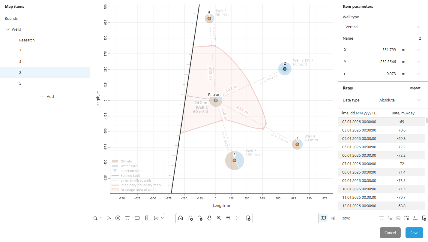
Around well 1 there are producers 3–5 and injector 2. To the west the area is bounded by a sealing fault.
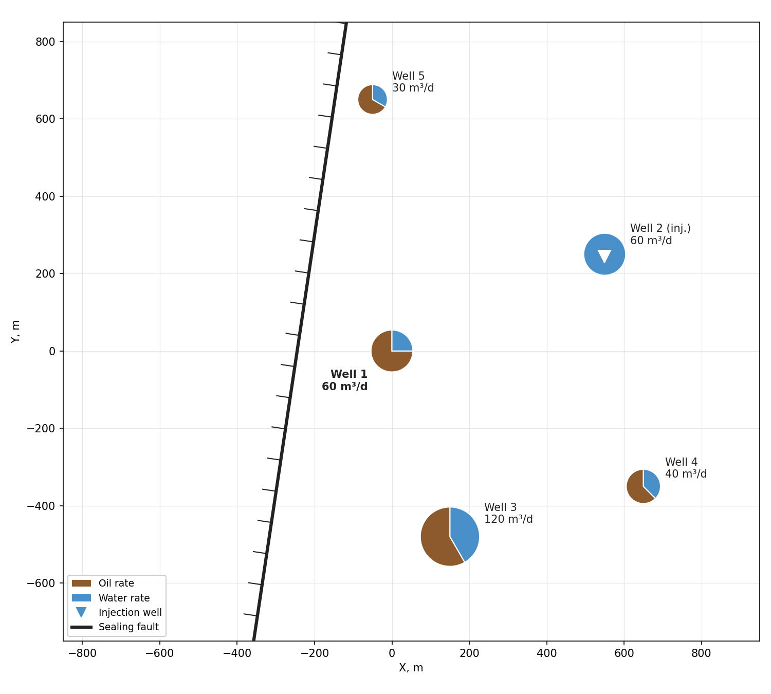
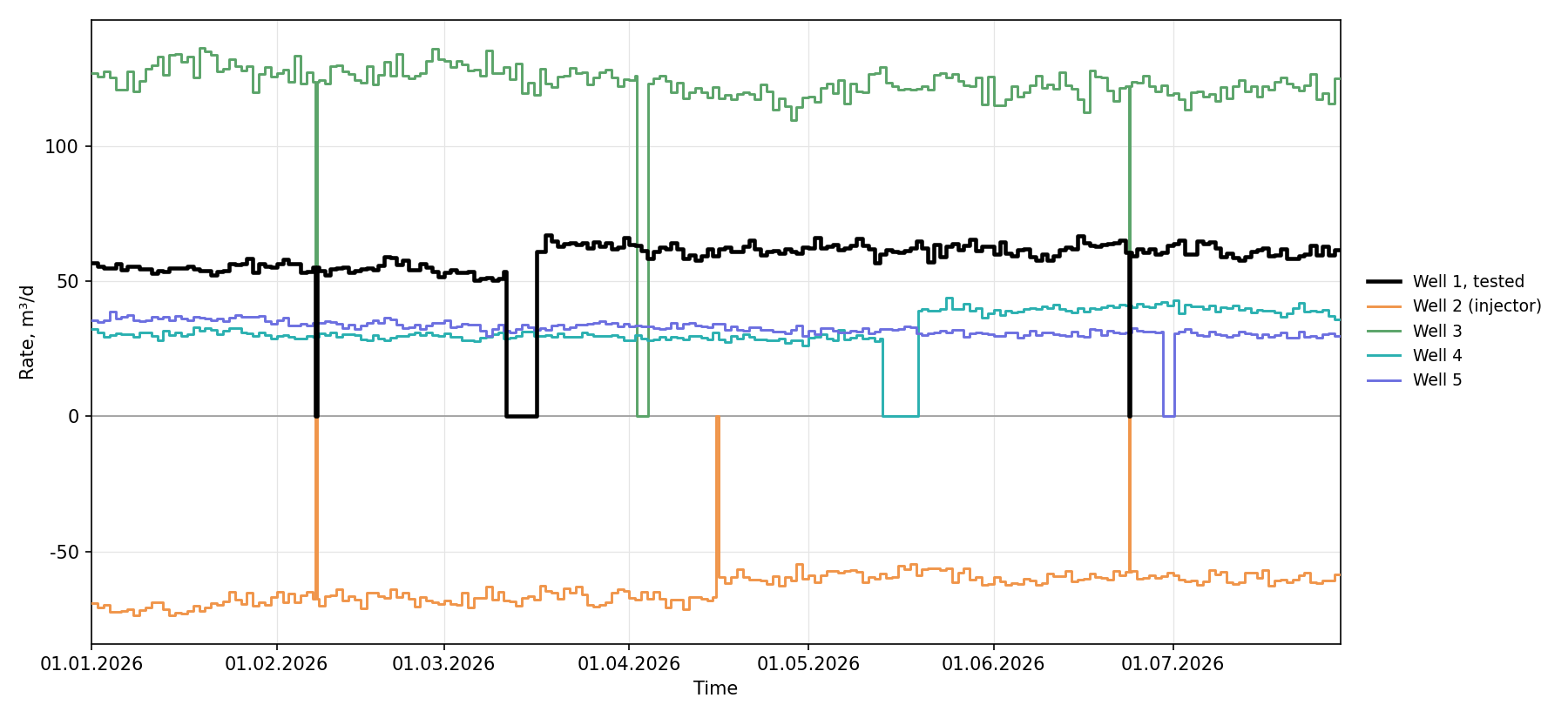
In the rapid design the well rates were taken as a single number from the current production map. In this case we work with more detailed data: the rates of the study well and the offset wells are taken from daily measurements in the well operating report. The operating history of the wells is shown in the plot below.
Analytical model
At the first stage we model only the study well. We do not include the offset wells in the model yet and account for their influence through boundaries.
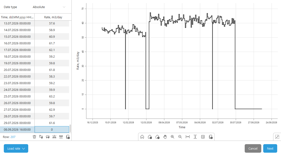
Rate history. We start with data input. In SiamWellTest we use the generation module and load the rate history of well 1. For this case we have data from January to July 2026. Let us assume that we are planning the PBU from this moment. At the end we add a long shut-in. We take its duration with a margin to follow the behavior of the whole curve and then decide from it how much time the test actually needs.
Base model. We enter the input data for the analysis from the table above: wellbore radius, thickness, porosity. The fluid properties are already available to us, so we simply enter them too. In real work they are usually calculated separately in the PVT module, see the article on PVT modeling for details.
Next we select a vertical well model in a homogeneous reservoir with constant WBS, without boundaries for now. We set the assumed system parameters: reservoir pressure 138 atm, permeability 30 mD, skin factor 0 and WBS coefficient 0.11 m³/atm.
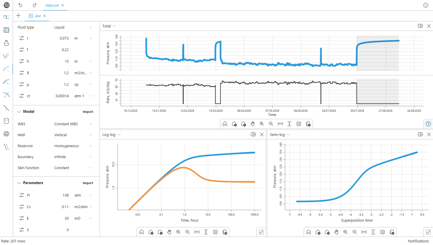
This gives us the basis for modeling. On the log-log plot, at the beginning of the PBU the pressure and the derivative follow the unit slope together: this is WBS. Then the derivative passes a hump with a peak at about 1 h and reaches the radial flow plateau by about 20 h. The reservoir in this model is infinite, so radial flow continues until the end of the shut-in.
Boundary model. The boundaries are determined from the current production map. The distance to the fault is measured along the perpendicular from the well. Offset wells create imaginary boundaries: wells of the same type (producers) create no-flow boundaries, wells of the opposite type (injectors) create constant pressure boundaries. The position of an imaginary boundary is found by dividing the distance between the wells in proportion to their rates:
where $L$ is the distance to the imaginary boundary, m; $D$ is the distance between the wells, m; $q_1$, $q_2$ are the current rates (injection rate) of the study well and the offset well, m³/d.
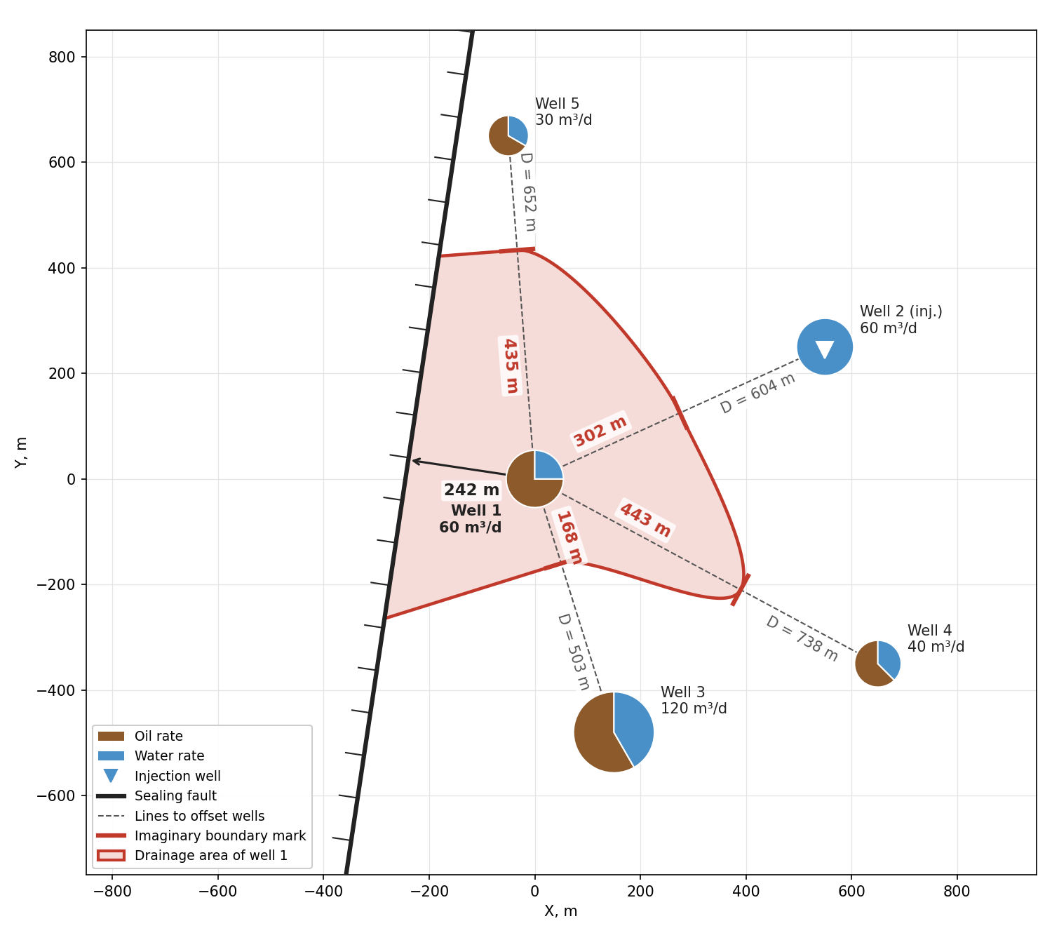
The well is surrounded by boundaries on all sides: the fault to the west and imaginary boundaries from the offset wells on the other sides. This means that the drainage area of well 1 is closed. With certain assumptions it can be approximated by a rectangle. For each of the four sides we take the nearest boundary. There are two to the east: from injector 2 (302 m) and from well 4 (443 m). The injector is closer, so we use it.
| Side | Boundary | Type | $L$, m |
|---|---|---|---|
| South | Well 3 | no-flow | 168 |
| West | Fault | no-flow | 242 |
| East | Well 2 (injector) | constant pressure | 302 |
| North | Well 5 | no-flow | 435 |
In SiamWellTest we select the "Rectangle" boundary model and enter the distances to the sides and their types. The other parameters are kept as in the base model, and we build the model PBU.
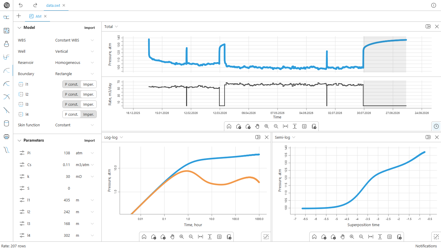
After 40–50 h the derivative goes up as the no-flow boundaries show up. After 400–500 h it goes down under the effect of the constant pressure boundary.
This is the first and simplest approximation that can be built with analytical tools. At early times it is exact: WBS, skin and radial flow do not depend on the boundaries. For interference, however, the model gives only an approximate estimate of when the effects will start to show. Quantitatively the picture will most likely turn out quite different.
The reason is that almost all boundaries in this model are imaginary, and imaginary boundaries behave differently from real ones. Their position depends on the rates of the offset wells and changes with them. Therefore, next we will try to account for the operation of the offset wells themselves.
Analytical interference model
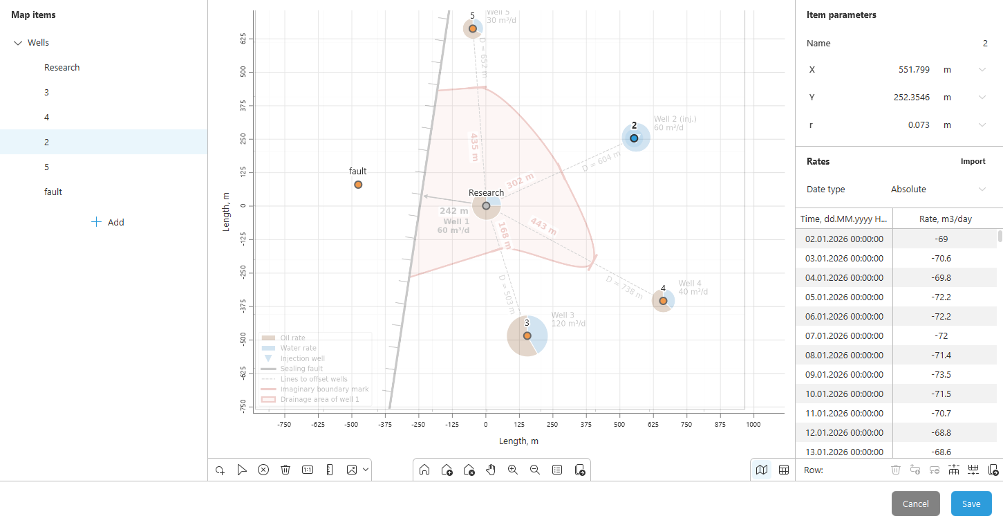
Now, instead of imaginary boundaries, we put the offset wells themselves into the model. To do this in SiamWellTest, we select the "Interference" type in the boundary model. This opens a map on which we place the offset wells.
Map. We place the study well at the center of the map and position offset wells 2–5 by their coordinates. Boundaries cannot be added here: analytical boundaries are built by reflecting wells, and with interference all the offset wells would have to be mirrored, which is practically unachievable in most cases. Therefore, in SiamWellTest a model is built either with boundaries or with offset wells.
To roughly account for the fault, we manually reflect only the study well: we place an image well with the same rate at twice the distance to the fault, 484 m from well 1.
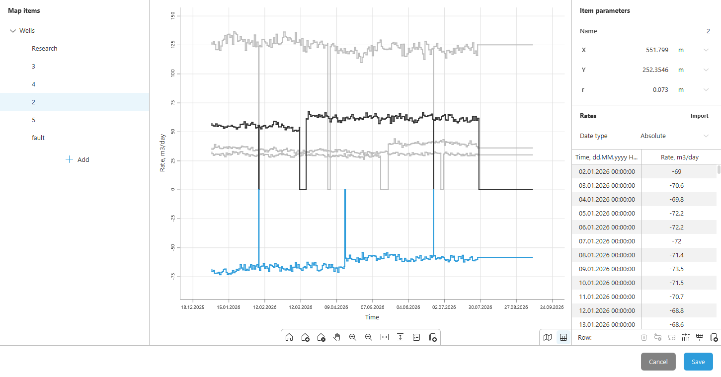
Rates. Each well on the map is given its rate history from the well operating report. Study well 1 and the image well behind the fault get the same history with the PBU shut-in at the end. We have no data on the operation of the offset wells during the PBU, so we extend their history for the same duration with the last measured rate.
Result. We keep the reservoir and well parameters unchanged and build the model PBU. To see what the transition from imaginary boundaries to real offset wells has given, we plot it on the same log-log plot as the boundary model.
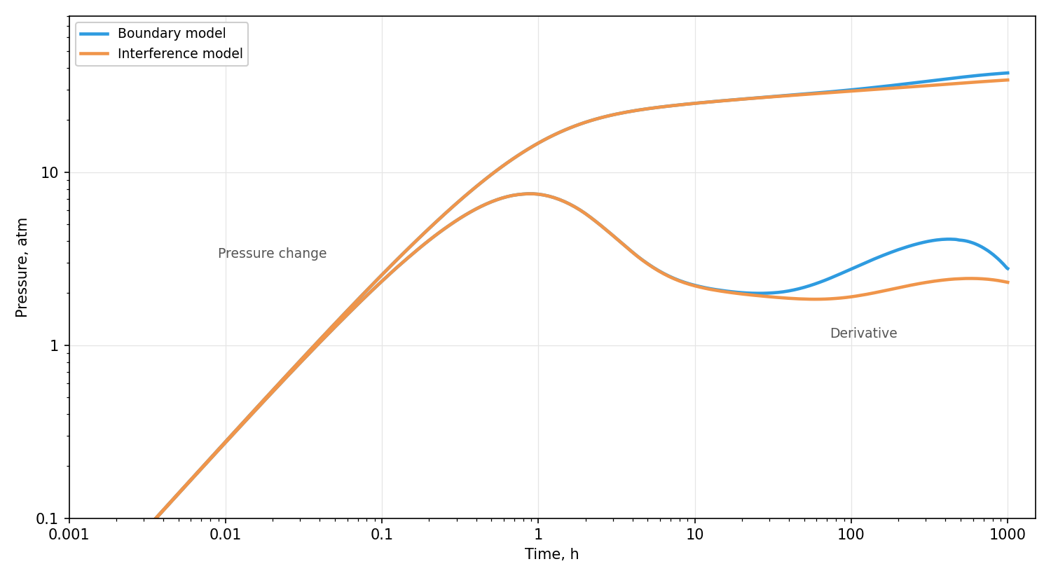
The picture is similar, but there are differences. The derivative stays near the plateau longer and goes up only after 100 h rather than after 40–50 h, and the rise is noticeably weaker. This difference is expected. The boundary model only approximates the influence of the offset wells with imaginary boundaries at a fixed distance. In the interference model the offset wells operate at their actual rates, so it reproduces their influence on the curve more accurately.
It should be noted, however, that this model is not perfectly accurate. The influence of the fault is set roughly: only the study well is reflected in it, and the reflections of the offset wells are not taken into account. For a more accurate forecast we move on to numerical modeling.
Numerical model
The numerical model removes the limitations of analytics: in it, both the offset wells and real boundaries of any shape can be set at the same time.
Map. We transfer the offset wells with their rate history from the interference model. The image well is no longer needed: we remove it and draw the fault at its actual position instead.
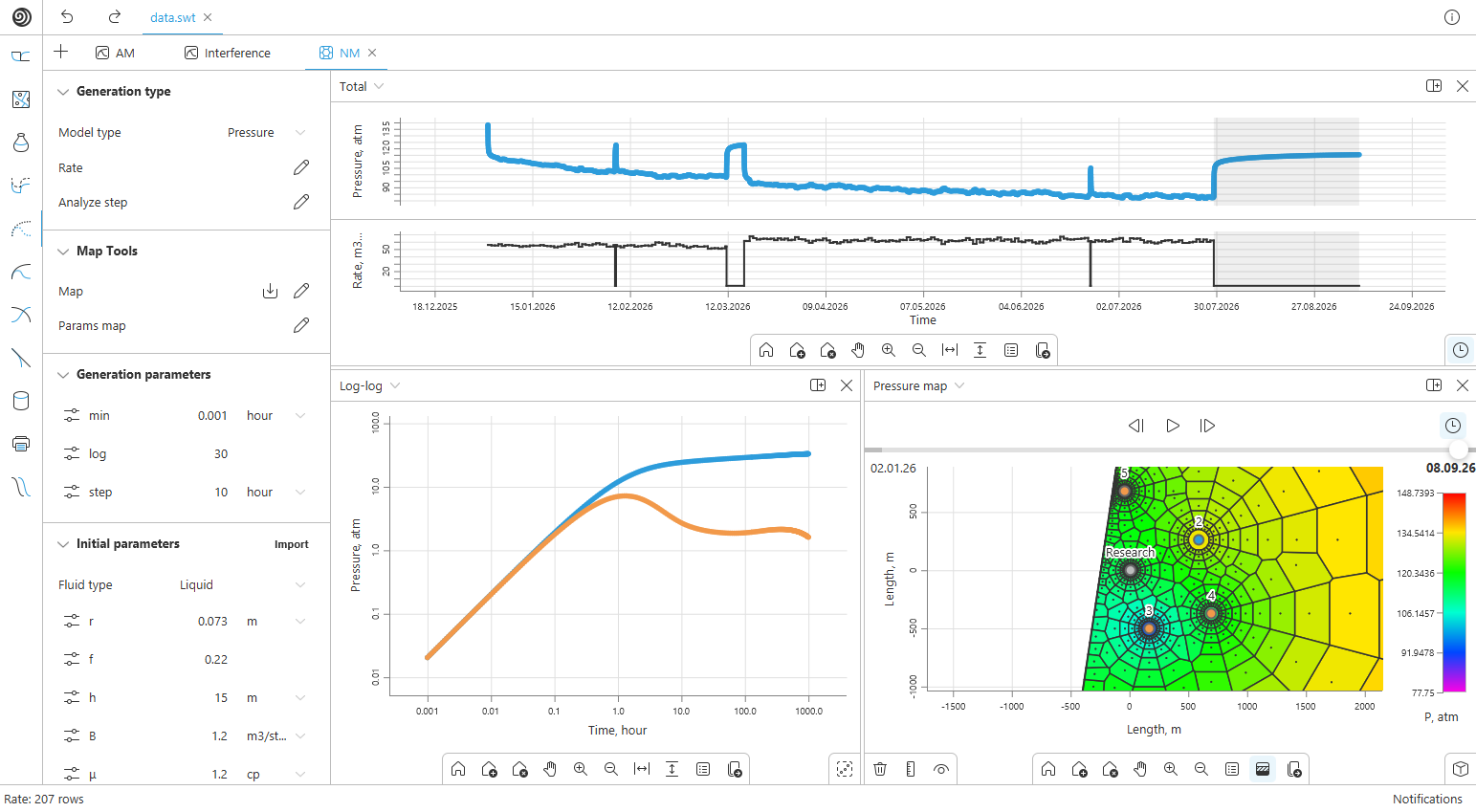
Simulation. We run the calculation. The pressure plot shows that the bottomhole pressure of well 1 gradually declines over the production period, and the pressure map shows a common depression cone around the producers, with the pressure in the area lower than far away from it. The injector does not compensate the withdrawal, so the decline of the derivative at the end of the PBU is caused not by a constant pressure boundary, as in the boundary model, but by the continuing withdrawal of the offset wells: the pressure builds up toward the area pressure, which falls with the withdrawal.
Result. We plot the model PBU of the numerical model on the same log-log plot as both analytical ones.
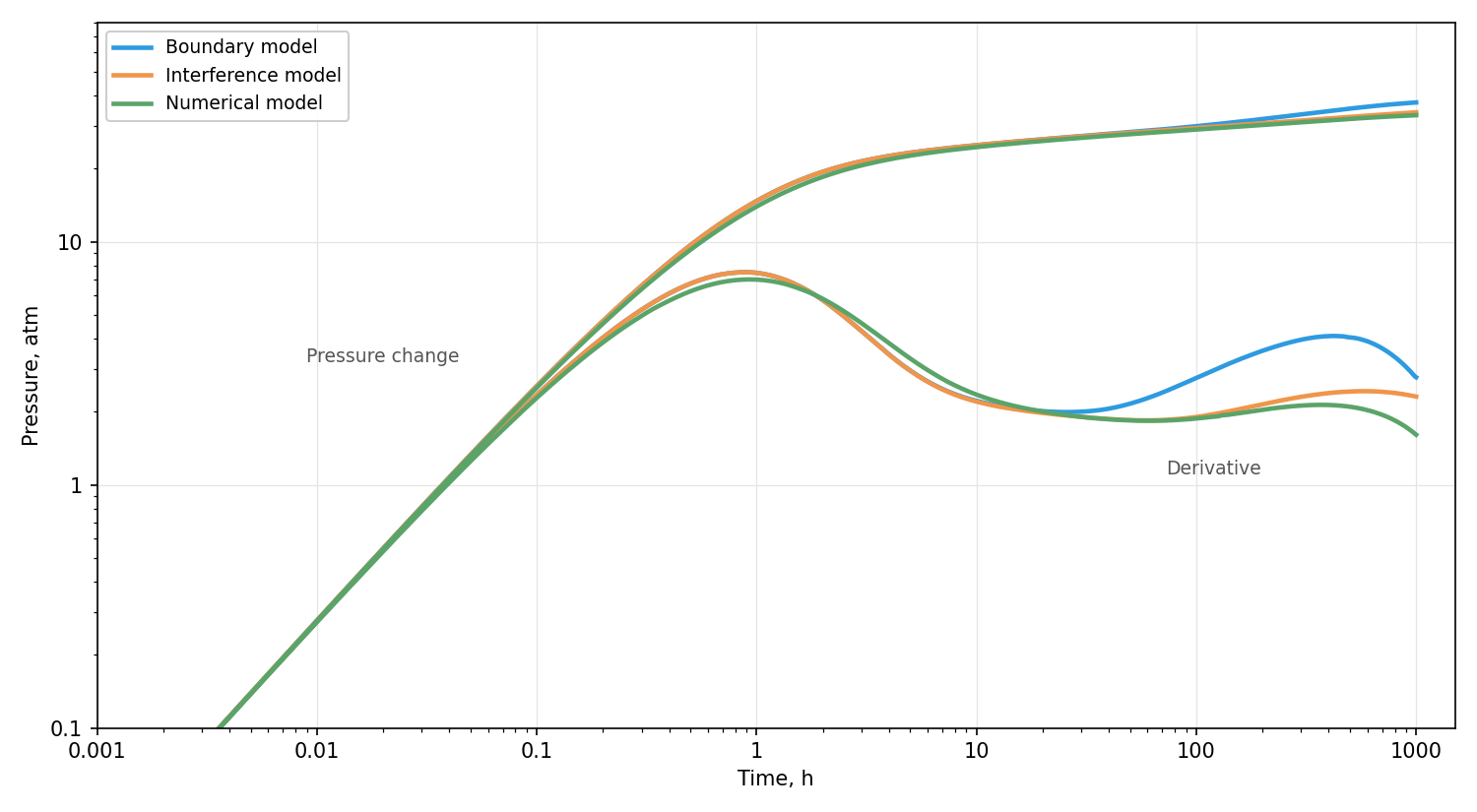
After radial flow is reached, the numerical model shows the same as the analytical interference model: the derivative stays near the plateau until about 100 h and then rises gently. The curves diverge only at late times, after 200–300 h: in the numerical model the derivative goes down earlier and more strongly.
The discrepancy with the analytical interference model is due to the rough representation of the fault in analytical modeling. In the numerical model the reservoir geometry and the operation of the offset wells are accounted for more correctly, so from here on we take its results as the reference.
Sensitivity analysis
Permeability, skin factor and WBS coefficient are the parameters the well test is meant to determine. We put their estimated values into the model, but the actual ones may differ noticeably and strongly affect the course of the test. Therefore, we take the numerical model as the base case and look at how the diagnostic plots change over the whole range of possible values.
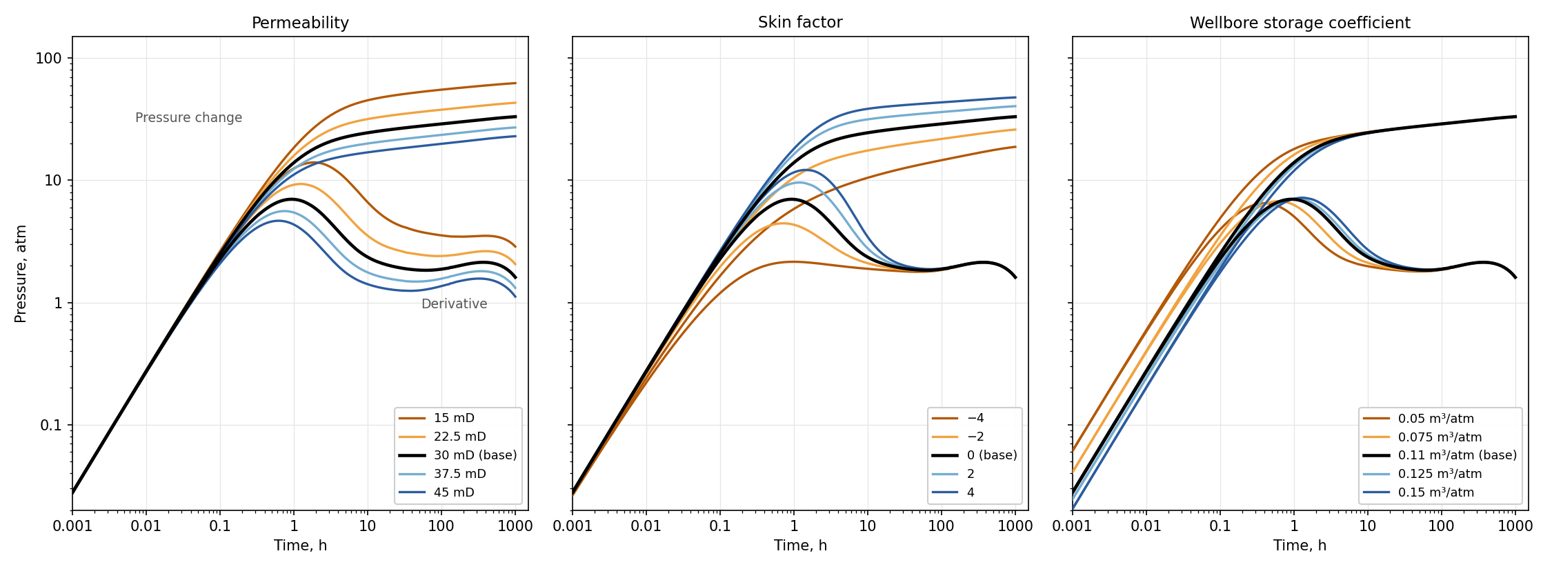
Permeability. We vary it from 15 to 45 mD. The parameter shifts the whole curve: the lower the permeability, the higher the whole curve and the later all effects occur. At 45 mD the offset wells show up already at about 90 h, at 15 mD only after 700 h. The radial flow window shifts to the right, while its width changes only slightly.
Skin factor. We vary it from −4 to +4. Skin affects only the beginning of the curve: the higher it is, the longer WBS lasts and the later radial flow begins. After the plateau is reached, the derivative curves coincide. Skin affects the test duration by setting its minimum. A high skin shortens the radial flow window, but in our range it does not close it.
WBS coefficient. We vary it from 0.05 to 0.15 m³/atm. The coefficient shifts the derivative hump in time: the larger it is, the later WBS ends and the more it overlaps the beginning of radial flow. But in our case, even at the largest value, radial flow remains visible.
Summary. In all cases radial flow is clearly identified, so the test is highly likely to be informative. However, the uncertainty in permeability results in uncertainty in the test duration, so we consider several scenarios.
| Scenario | $k$, mD | Radial flow, h | Radial flow duration, log cycles | Shut-in duration, h | Oil production loss, m³ |
|---|---|---|---|---|---|
| Pessimistic | 15 | 40–750 | 1.28 | 360* | 680* |
| Base | 30 | 22–180 | 0.92 | 180 | 340 |
| Optimistic | 45 | 15–90 | 0.80 | 90 | 170 |
\* At low permeability radial flow lasts longer than needed for interpretation. Recording about one log cycle is enough, as in the base scenario, so the shut-in ends at 360 h without waiting for the offset wells to show up.
The shut-in duration in the table is taken as the end of radial flow. The oil production loss during the shut-in is calculated for the current liquid rate of 60 m³/d and a water cut of 25 %:
where $Q_o$ is the oil production loss, m³; $q$ is the liquid rate, m³/d; $W$ is the water cut, fraction; $t$ is the shut-in duration, h.
Conclusions
Design results:
- the test will be informative for any plausible parameters: radial flow is identified in all cases;
- in the base scenario the shut-in will take no more than 180 h, and the production loss will be about 340 m³ of oil;
- depending on the actual permeability, the shut-in will take from 90 to 360 h, and the loss from 170 to 680 m³.
Approaches:
- Boundary model. The fastest way to assess whether a test is feasible: working with the study well alone is enough, boundaries are set as numbers and are convenient to adjust with sliders in real time. Drawback: the model is accurate only at early times, while at late times the influence of the surroundings through imaginary boundaries is estimated only approximately, with errors.
- Interference model. Accurately estimates the influence of offset wells in the absence of geological boundaries. If they are present, modeling is possible, but with assumptions and errors. It computes an order of magnitude faster than numerical models. Drawback: complex reservoir geometry cannot be built.
- Numerical model. Allows any reservoir geometry to be set and accurately accounts for both the operation of the offset wells and the geology. It stores the pressure fields of the whole object: you can study how pressure behaves throughout the reservoir. Drawback: a heavier tool that requires more preparatory work, and the computation time of such models is an order of magnitude longer than that of analytical models.
All stages of the case were done in a single SiamWellTest project. You can read more about the software on the product page.