Goal. Show how to estimate the prospects and duration of a pressure build-up (PBU) test without a simulator, using simple analytical expressions, with the free mobile app SiamEngy as an example.
Audience. This document is intended for three groups of readers:
- well test engineers who plan tests: the material lets you learn or reproduce the rapid design method;
- field engineers who prepare test programs and shut in wells: the approach lets you estimate test durations across the entire well stock on your own and check the timing built into well test programs;
- engineers from related disciplines and managers whose work is connected with well testing: for a general understanding of what determines the shut-in time and the production losses when wells are shut in for testing.
What we do. We go through an end-to-end calculation example in SiamEngy and compare the result with a reference model in a simulator. The theoretical basis of the rapid method is collected in the appendix at the end of the article.
Study object
We are planning a PBU on an oil producer. The well is vertical and produced by an electric submersible pump (ESP). We have the well operating report, the field development plan, the well log interpretation, the PVT report, the isobar map and the current production map. Below we extract from them the parameters needed for the design.
Well operating report. From the well operating report we take the current operating conditions of the well and its design. From the well design we will calculate the annulus cross-section area, and from it and the liquid density, the wellbore storage (WBS) coefficient.
| Parameter | Value |
|---|---|
| Production method | ESP |
| Liquid rate, $q$ | 60 m³/d |
| Water cut | 25 % |
| Liquid density, $\rho$ | 850 kg/m³ |
| Production casing | 146 mm |
| Casing inner diameter | 130 mm |
| Tubing | 73 mm |
| Wellbore radius, $r_w$ | 0.073 m |
| Perforation interval (TVD) | 1,462–1,478 m |
Field development plan. Porosity and permeability are taken from the table of geological and physical properties of the production target. The permeability at the well is not known in advance: this is exactly what the test is meant to determine. For the design we take the average value for the target. If more reliable sources are available, for example well test results from offset wells, it is better to take the permeability from there.
| Parameter | Value |
|---|---|
| Porosity, $\phi$ | 0.22 |
| Permeability, $k$ | 30 mD |
Well log interpretation. The net pay thickness at the well is taken from the well log interpretation report.
| Parameter | Value |
|---|---|
| Net pay thickness, $h$ | 15 m |
PVT report. From the PVT report we take the fluid and system properties at reservoir conditions.
| Parameter | Value |
|---|---|
| Formation volume factor, $B$ | 1.2 m³/m³ |
| Viscosity, $\mu$ | 1.2 cP |
| Total compressibility, $c_t$ | 1.4·10⁻⁴ atm⁻¹ |
Isobar map. The current reservoir pressure around the well is read from the isobar map.
| Parameter | Value |
|---|---|
| Reservoir pressure, $P_r$ | 138 atm |
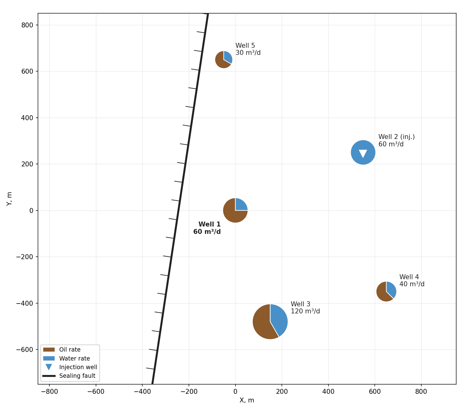
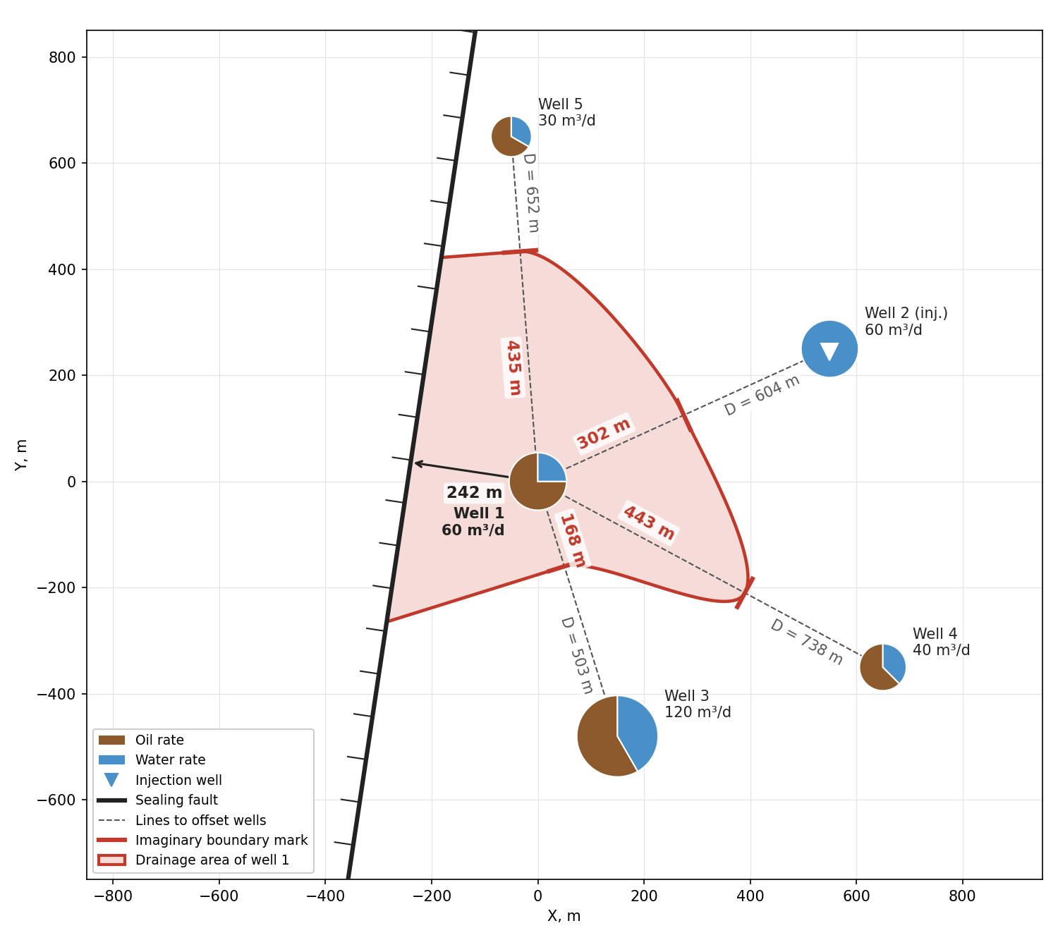
Current production map. Around the study well (well 1) there are producers 3–5 and injector 2. To the west the area is bounded by a sealing fault. We will use the map to determine the distances to the boundaries that may show up on the PBU.
Skin factor. The skin factor is one of the parameters the test is run for, so we do not have its exact value. However, it can be estimated from the well intervention history. For example, if the well has had acid treatments or hydraulic fracturing, a negative skin can be assumed, and after well kills and workovers that damaged the near-wellbore zone, a positive one. Still, such an estimate remains approximate, so it is more reliable to check the sensitivity of the forecast to skin. This is what we will do: in the base case we take $s = 0$, and other values are considered in the sensitivity analysis.
The design needs two times: when radial flow begins and when the nearest boundary starts to affect the response. The first is determined by the end of WBS, the second by the distance to the boundary.
WBS coefficient
The well is equipped with an ESP. After the pump is stopped, the inflow from the reservoir goes into raising the liquid level in the annulus, so WBS is governed by the changing liquid level. The annulus cross-section area $S$ is calculated from the casing inner diameter $D_c$ and the tubing outer diameter $d_t$:
In SiamEngy we select the formula "WBS coefficient for pumping well" and enter the cross-section area, the liquid density and the wellbore angle. For our vertical well the angle is zero.
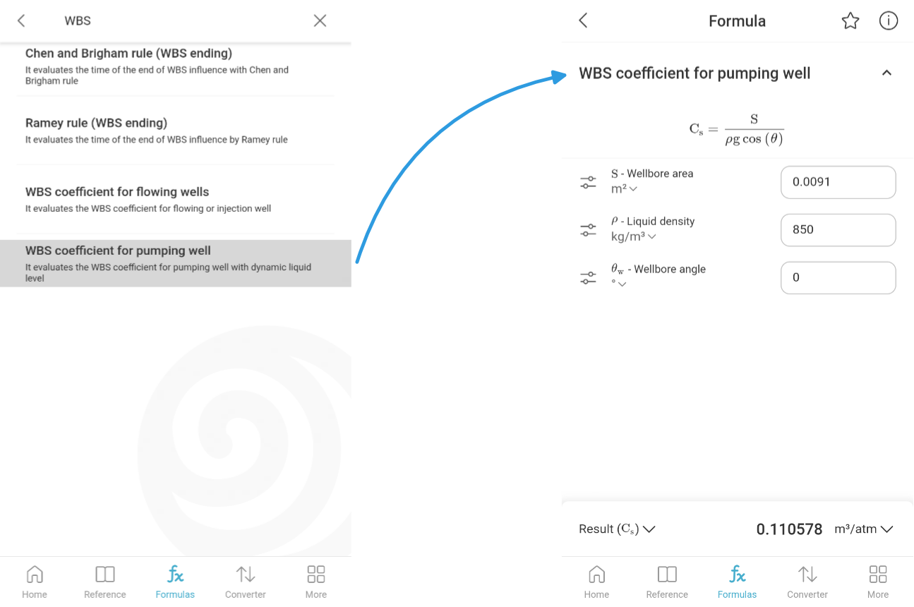
We get a WBS coefficient of $C \approx 0.11$ m³/atm. This is a typical value for wells on artificial lift.
Start of radial flow
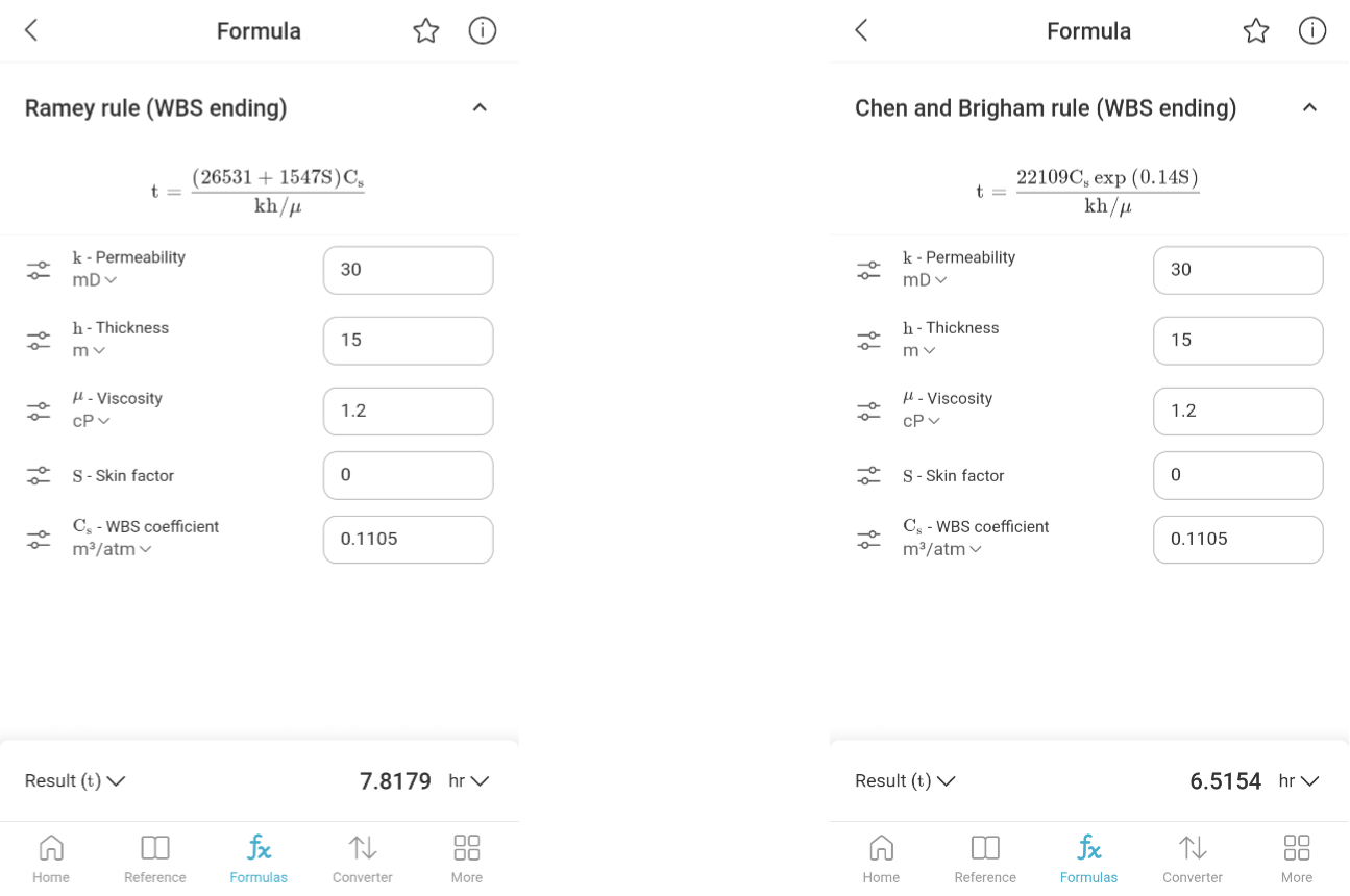
The well is vertical, so radial flow begins right after the end of WBS. The end of WBS is estimated with two empirical rules: Ramey's and Chen–Brigham's. In both SiamEngy formulas we enter permeability, thickness, viscosity, skin factor and the WBS coefficient obtained above.
| Rule | Start of radial flow |
|---|---|
| Ramey | 7.8 h |
| Chen and Brigham | 6.5 h |
The rules give similar values. For further calculations we take the larger one, 7.8 h: in test design it is better to err on the side of a later start of radial flow.
Nearest boundary
The distances to the boundaries are determined from the current production map. The distance to the fault is measured along the perpendicular from the well. Between well 1 and each offset well we draw a straight line and place an imaginary boundary mark in proportion to the rates:
where $L$ is the distance to the mark, m; $D$ is the distance between the wells, m; $q_1$, $q_2$ are the liquid rates (injection rate) of the study well and the offset well, m³/d.
| Boundary | Type | $D$, m | $q_2$, m³/d | $L$, m |
|---|---|---|---|---|
| Well 3 | no-flow | 503 | 120 | 168 |
| Fault | no-flow | — | — | 242 |
| Well 2 (injector) | constant pressure | 604 | 60 | 302 |
| Well 5 | no-flow | 652 | 30 | 435 |
| Well 4 | no-flow | 738 | 40 | 443 |
The nearest boundary is the flow divide with well 3 at a distance of 168 m. It is potentially the first one to distort radial flow.
Note. If there is no current production map, the drainage radius can be used instead of the distance to the nearest boundary: it is usually available in the well operating report. The estimate will be rough, but it is good enough as a first approximation. The drainage radius is also convenient for bulk calculations across the entire well stock in Excel.
Onset of boundary effect
The onset of the boundary effect is calculated with the radius of investigation formula. It is important to note that a radius of investigation equal to the distance to the boundary is only the moment when its influence begins. On the derivative the boundary becomes noticeable later, so in practice a factor of 1.5 is applied to the distance. More on this in the appendix. In our case we use $1.5 \cdot 168 \approx 252$ m.
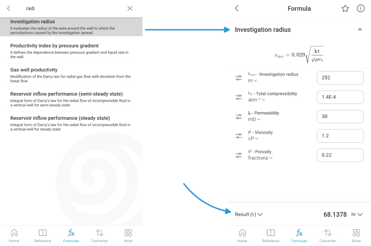
SiamEngy has a radius of investigation formula, and in it you can choose which parameter to calculate. We choose time $t$ as the result and enter 252 m in the radius of investigation field. We get $t \approx 68$ h.
Base estimate of test duration and production losses
Radial flow begins at 7.8 h and the boundary effect at 68 h. The duration of radial flow is estimated in log cycles:
where $N$ is the number of log cycles; $t_b$ is the onset of the boundary effect, h; $t_r$ is the start of radial flow, h.
A long radial flow period is expected, almost a full log cycle. This is enough to reliably determine permeability and skin factor.
The test duration is taken equal to the onset of the boundary effect, 68 h. Oil production losses during the shut-in:
where $Q_o$ is the oil production loss, m³; $q$ is the liquid rate, m³/d; $W$ is the water cut, fraction; $t$ is the test duration, h.
Sensitivity analysis
Permeability and skin factor are exactly the parameters the test is run for, so they are known only approximately in advance. Let us check how the forecast changes if they differ from the assumed values: permeability by ±25 and ±50 %, skin factor by ±2 and ±4. For each combination we repeat the calculation and get the length of the radial flow window in log cycles and the test end time in hours.
How to read the table: rows are permeability, columns are skin factor. Each cell shows, separated by a slash, the length of the radial flow window in log cycles / the test end time in hours. The base case is in bold.
| $k$, mD | $s = -4$ | $s = -2$ | $s = 0$ | $s = 2$ | $s = 4$ |
|---|---|---|---|---|---|
| 15 (−50 %) | 1.06 / 136 | 1.00 / 136 | 0.94 / 136 | 0.89 / 136 | 0.78 / 136 |
| 22.5 (−25 %) | 1.06 / 91 | 1.00 / 91 | 0.94 / 91 | 0.89 / 91 | 0.78 / 91 |
| 30 | 1.06 / 68 | 1.00 / 68 | 0.94 / 68 | 0.89 / 68 | 0.78 / 68 |
| 37.5 (+25 %) | 1.06 / 55 | 1.00 / 55 | 0.94 / 55 | 0.89 / 55 | 0.78 / 55 |
| 45 (+50 %) | 1.06 / 45 | 1.00 / 45 | 0.94 / 45 | 0.89 / 45 | 0.78 / 45 |
The window length depends only on the skin factor. Skin affects the start of radial flow: the higher it is, the longer WBS lasts. The onset of the boundary effect does not depend on skin, so as skin increases the window narrows from 1.06 to 0.78 log cycles. Permeability does not affect the window length: both the start of radial flow and the onset of the boundary effect are inversely proportional to permeability, so the whole window shifts in time.
The end time, on the contrary, depends only on permeability: from 45 h at $k = 45$ mD to 136 h at $k = 15$ mD. When permeability is 50 % lower, the shut-in duration doubles.
The test is robust to parameter uncertainty: in all cases radial flow lasts at least 0.78 log cycles, and the test should be informative. So it can be carried out. The main uncertainty is in the duration: depending on permeability it may range from 45 to 136 h, and the production losses from 85 to 255 m³ of oil. Therefore, the plan should include a time margin, and it should be decided in advance whether such losses are acceptable.
Comparison with numerical simulation
To check the rapid estimate, we build a numerical model of the area in the SiamWellTest simulator: the same reservoir and fluid properties, WBS coefficient, fault and offset wells with their rates. We simulate a long production period of well 1 followed by a long PBU shut-in to follow the behavior of the whole curve.
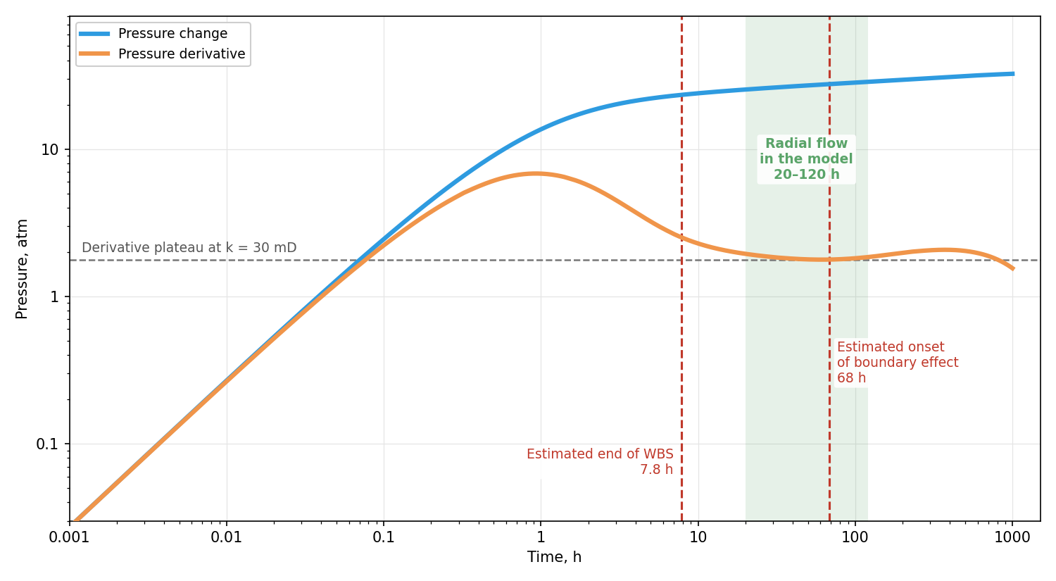
Radial flow corresponds to a horizontal plateau of the derivative. Its level is set by the reservoir permeability: the plot shows the plateau given by the 30 mD permeability used in the model. The derivative reaches the plateau at about 20 h and stays on it until 120 h, which is 0.78 log cycles. After that the derivative leaves the plateau as the boundaries start to show.
| Parameter | Rapid estimate | Model |
|---|---|---|
| Start of radial flow | 7.8 h | 20 h |
| Onset of boundary effect | 68 h | 120 h |
| Radial flow duration | 0.94 log cycles | 0.78 log cycles |
On the log-log plot the rapid estimate and the model agree satisfactorily. The estimated radial flow window is close in size to the model one but shifted to the left: the rapid estimate underestimated both the end of WBS and the onset of the boundary effect. On a log scale this shift is small, but in hours it is noticeable: the boundary shows up at 120 h rather than 68 h. Overall, however, the picture is the same, and the model confirms that the test will be informative.
For a method of this level, such a discrepancy is the norm rather than the exception, since it is based not on exact calculations but on approximate empirical rules. This should be kept in mind when applying it: the rapid estimate gives the order of magnitude and the likelihood that the test will be informative, not exact numbers.
Conclusions
We went through an end-to-end example of rapid PBU design for a vertical well. It showed that without a simulator, using a few analytical formulas and data available in any field, it is possible to estimate the prospects and duration of a test. The same method applies to fractured and horizontal wells, with a correction for their geometry.
The comparison with the numerical model confirmed that the method is reasonably accurate, but only to an order of magnitude. It answers the qualitative question, whether the test will be informative, fairly reliably. The quantitative estimates, shut-in duration and production losses, are approximate and should be included in the plan with a margin.
The main advantage of the method is speed and scale. The formulas are simple: they can be built directly into the well operating report spreadsheet in Excel and extended to all wells. The entire well stock is processed in a few minutes: for each well we get the test duration and production losses, and use them to rank the candidates. You can explore the formulas or try the calculation in the free SiamEngy app (Google Play, App Store).
One sensible strategy is to use the rapid method for bulk screening and then analyze the selected candidates in detail with numerical models in simulators, for example in SiamWellTest.
Appendix. Theoretical basis of the rapid method
In the practical part all calculations were done in SiamEngy. Here we collect the formulas behind them. They can be transferred to Excel and applied to the entire well stock. We also discuss the justification of the 1.5 factor and the specifics of fractured and horizontal wells.
Formulas
WBS coefficient. If the wellbore is completely filled with liquid, WBS is governed by its compressibility; if the level rises after shut-in, as in wells on artificial lift, it is governed by the cross-section area in which the level moves:
where $c_{wb}$ is the compressibility of the fluid in the wellbore, atm⁻¹; $V_{wb}$ is the wellbore volume, m³; $S$ is the cross-section area, m²; $\rho$ is the density of the fluid in the wellbore, kg/m³; $g$ is the gravitational acceleration, m/s².
The WBS coefficient due to a changing level is one to two orders of magnitude larger, so in wells on artificial lift WBS often determines the duration of the entire test.
End of WBS. The Ramey [1] and Chen–Brigham [2] rules in dimensionless form:
where $t_D$ and $C_D$ are the dimensionless time and WBS coefficient; $s$ is the skin factor.
In dimensional form:
where $t$ is the end of WBS, h; $C$ is the WBS coefficient, m³/atm; $\mu$ is the viscosity, cP; $k$ is the permeability, mD; $h$ is the net pay thickness, m.
Radius of investigation and the inverse formula, the time it takes to reach a distance $r$:
where $r$ is the radius of investigation, m; $t$ is the time, h; $k$ is the permeability, mD; $\phi$ is the porosity, fraction; $\mu$ is the viscosity, cP; $c_t$ is the total compressibility, atm⁻¹.
In SiamEngy the same formula is written in US oilfield units with a coefficient of 0.029 [3]. Other coefficients can be found in the literature: the radius of investigation is a conventional concept, and different authors define it differently. The 1.5 factor below refers specifically to this formula.
The 1.5 factor
In practice, the onset of the boundary effect calculated from the distance itself usually comes out earlier than the actual one. The reason lies in the nature of the formula. The radius of investigation shows how far the pressure disturbance has propagated, that is, it corresponds to the moment when the boundary only begins to affect the pressure at the well. At that moment the derivative deviates from the radial flow plateau by only a few percent. On real data such a deviation is lost in the noise, and the boundary becomes visible noticeably later.
The plot collects models of wells with boundaries for various reservoir and fluid parameters. At a radius of investigation equal to the distance to the boundary, the derivative is only beginning to deviate. Such a change is hard to notice on real data. At a radius of 1.5 times the distance, the deviation is already clearly visible.
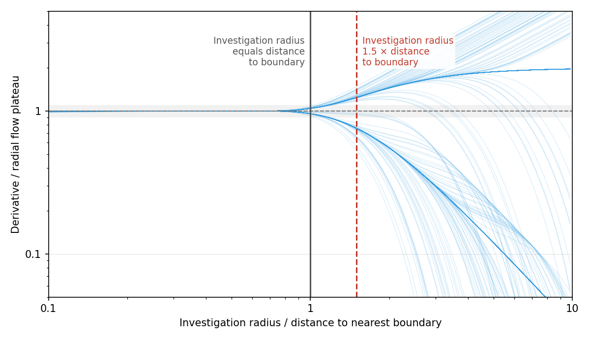
In addition, in practice boundary effects are often created not by true boundaries such as faults but by offset wells. On the derivative such effects appear differently than a single boundary. Experience shows that the 1.5 factor averages such cases well and works in practice.
Nevertheless, the choice of the factor is largely a matter of taste. For your own fields, taking into account the quality of the measurements, you can choose your own.
Hydraulic fracture and horizontal wellbore
In a well with a hydraulic fracture or a horizontal wellbore, radial flow does not begin immediately after the end of WBS. First, flow is toward the fracture or the wellbore, and only when the drainage area grows noticeably larger than their size does it become pseudo-radial. This moment is also estimated from the radius of investigation.
The same feature applies here as with boundaries: the time calculated from the fracture or wellbore length itself comes out shorter than the actual one. When the radius of investigation equals the length of the geometry, flow in the reservoir is still transitional, and radial flow has not yet begun.
The plot collects models of horizontal wells for various reservoir, fluid and wellbore parameters. At a radius of investigation equal to the wellbore length, the derivative has not yet reached radial flow. At a radius of 1.5 times the length, it is practically there.
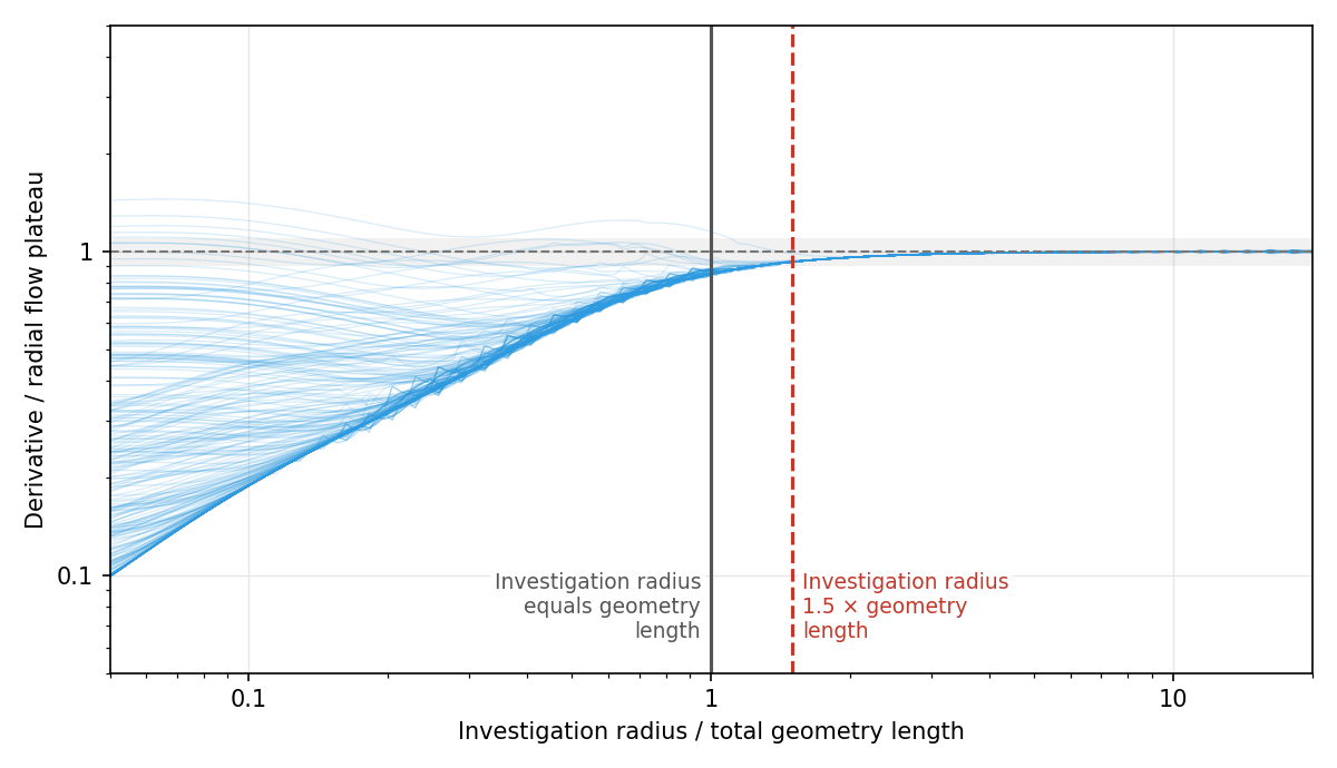
At late times a hydraulic fracture behaves the same way as a horizontal wellbore of the same length. Therefore, the rule is the same for both: a factor of 1.5 applied to the full length of the geometry.
| Geometry | Full length | Distance in the formula |
|---|---|---|
| Hydraulic fracture | $2\,x_f$ | $3\,x_f$ |
| Horizontal wellbore | $L$ | $1.5\,L$ |
The start of radial flow for such a well is the larger of two times: the end of WBS and the time from the radius of investigation. With a large WBS coefficient and a short fracture, the geometry may be completely masked by WBS, while for a long fracture or wellbore in a low-permeability reservoir, radial flow begins much later than the end of WBS.
References
- Ramey, H.J. Jr. 1970. Short-Time Well Test Data Interpretation in the Presence of Skin Effect and Wellbore Storage. Journal of Petroleum Technology 22 (1): 97–104.
- Chen, H.-K. and Brigham, W.E. 1978. Pressure Buildup for a Well With Storage and Skin in a Closed Square. Journal of Petroleum Technology: 141–146.
- van Poollen, H.K. 1964. Radius-of-Drainage and Stabilization-Time Equations. Oil and Gas Journal.