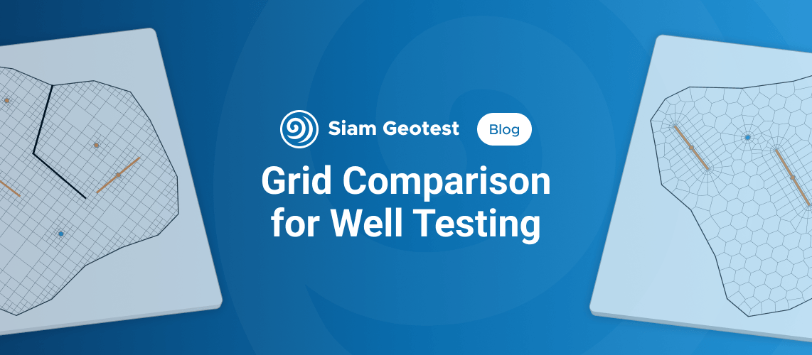
If you have ever used numerical models for well testing, you have most likely worked with a Voronoi grid. This approach has become the de facto standard in well testing. But why did things turn out this way? Let's work through it together.
The role of numerical models in well testing
In well testing, we use models to calculate pressure at a point. In essence, this is the only point in space where accuracy matters to us. We can simplify details elsewhere in the system, provided those simplifications do not affect the accuracy of the calculation in the area of interest.
At the same time, we want the calculations to be as fast as possible, so that we can test as many hypotheses as possible in the time available.
These two principles set the conditions that guide the practical choice of both the grid and the numerical solver.
Choosing a calculation grid
There are many types of calculation grids. Our context sets the requirements: calculate pressure at a single target point as accurately and as quickly as possible. We therefore need a grid that can represent any geometry while allowing us to vary the level of detail where needed. The grid generation algorithm should be as simple as possible, the solver should run as quickly as possible on that grid, and the number of cells should be kept to a minimum. Using these criteria, we will focus on the following types:
- Adaptive Cartesian grid
- Adaptive triangular grid
- Unstructured All-Quad grid
- Voronoi grid
We exclude several other common grid types from the comparison for the following reasons:
- Conventional structured grids. In regular grids, refinement around wells, faults and boundaries inevitably extends along coordinate lines across the entire domain, producing many unnecessary cells. The resulting increase in problem size offsets the high calculation speed. This is a serious drawback for well testing, where the objects being studied often have a highly heterogeneous structure.
- Curvilinear grids. This class of grids has been studied extensively for reservoir modeling. In practice, however, it struggles with complex fault geometries and is difficult to refine locally. It is considerably less flexible and harder to automate than adaptive and unstructured approaches.
- Corner-point grids. These grids are used in full-field 3D modeling to represent complex vertical reservoir geology in detail. For well test interpretation, this approach is excessive.
Adaptive Cartesian grid
This type of grid is generated using a square template. Where we do not need detail, we can use a larger template. Where detail is needed, we subdivide the template recursively. It is a very simple algorithm that can represent any geometry to the required accuracy.
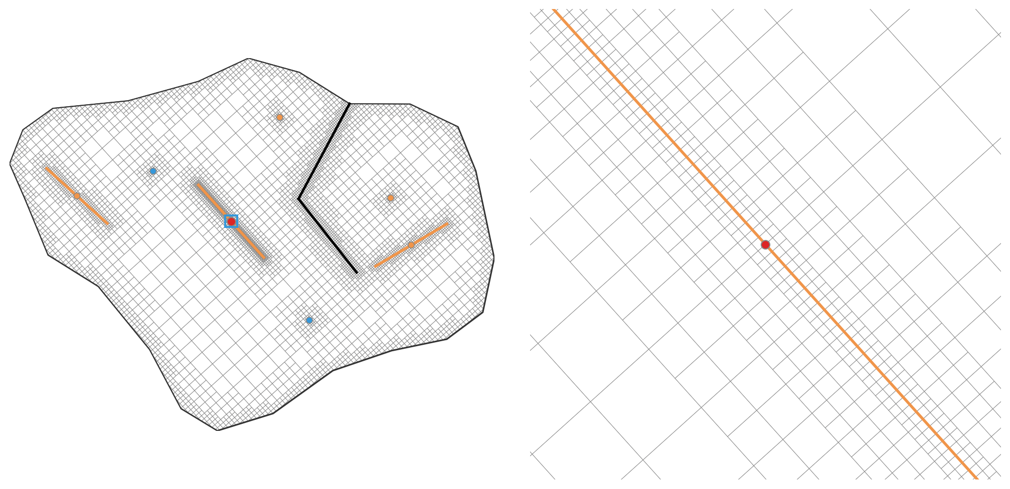
One drawback of this approach is the large number of cells, which ultimately affects calculation speed. However, simpler calculations partly offset this drawback. The regularity of the cells removes the need to store complex face geometry and allows us to use fast stencil-based algorithms instead of computationally expensive calculations for arbitrary polygons.
Adaptive triangular grid
We consider this grid as an alternative to the Cartesian grid, built using a triangular template. Where refinement is needed, each element is divided at its edge midpoints into four smaller triangles with half the edge length. Because the edges run in three directions, this grid can approximate complex parts of the model more accurately and with fewer stair steps.
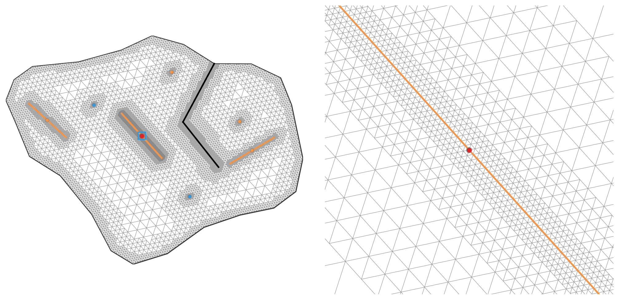
Despite their similar basic properties, triangular grids have two main disadvantages compared with square grids in flow simulations. First, they can violate orthogonality between cell-center connections and shared faces, reducing accuracy and slowing convergence. Second, they require more elements at the same refinement level. The result is slower calculation, as we will see in the practical comparison.
Unstructured All-Quad grid
This grid consists of quadrilaterals whose shapes and sizes adapt to the model geometry. Unlike a Cartesian grid, it has no single square template. Cell edges can change direction, allowing the grid to represent arbitrary configurations of the reservoir, faults and fractures. We concentrate small cells around wells and fractures and use coarser cells farther away.
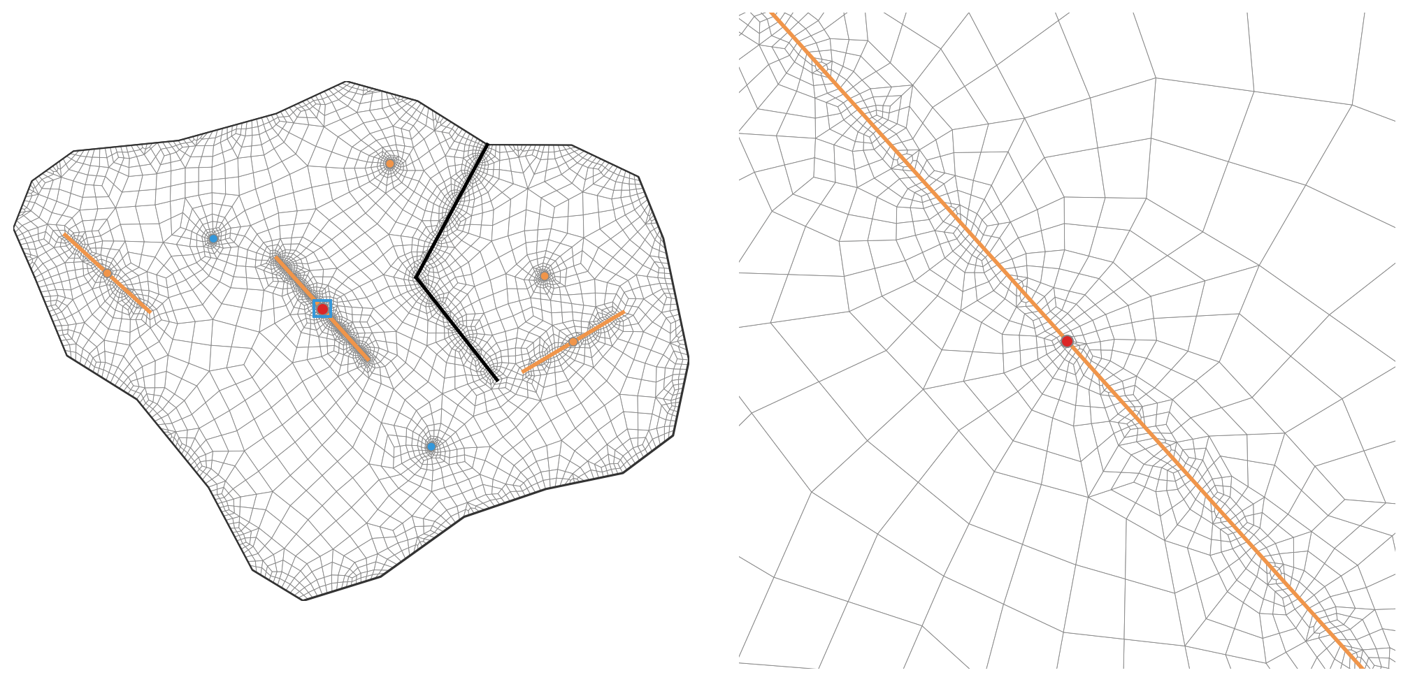
At first glance, this looks like a good compromise: the cells remain quadrilateral, and their total number is smaller than in the Cartesian grid. In practice, however, the approach faces two serious problems. First, generating a conforming quadrilateral grid that follows arbitrary geometry is more difficult than recursively subdividing squares or triangles. Second, arbitrary cell shapes do not guarantee orthogonality between cell-center connections and shared faces, which affects both accuracy and calculation speed.
Voronoi grid
This approach differs fundamentally from those discussed above. Conventional grids impose a cell shape and rules for connecting the cells. A Voronoi grid works differently. We specify the generating points, and the Voronoi algorithm constructs the cells around them.
This gives us complete freedom to control grid density. We can place the generating points in the plane according to the physics of the problem, packing them closely around the study well and spacing them widely at the periphery. We are free from a fixed cell shape and can represent highly complex boundary and fault geometries with relatively few elements.
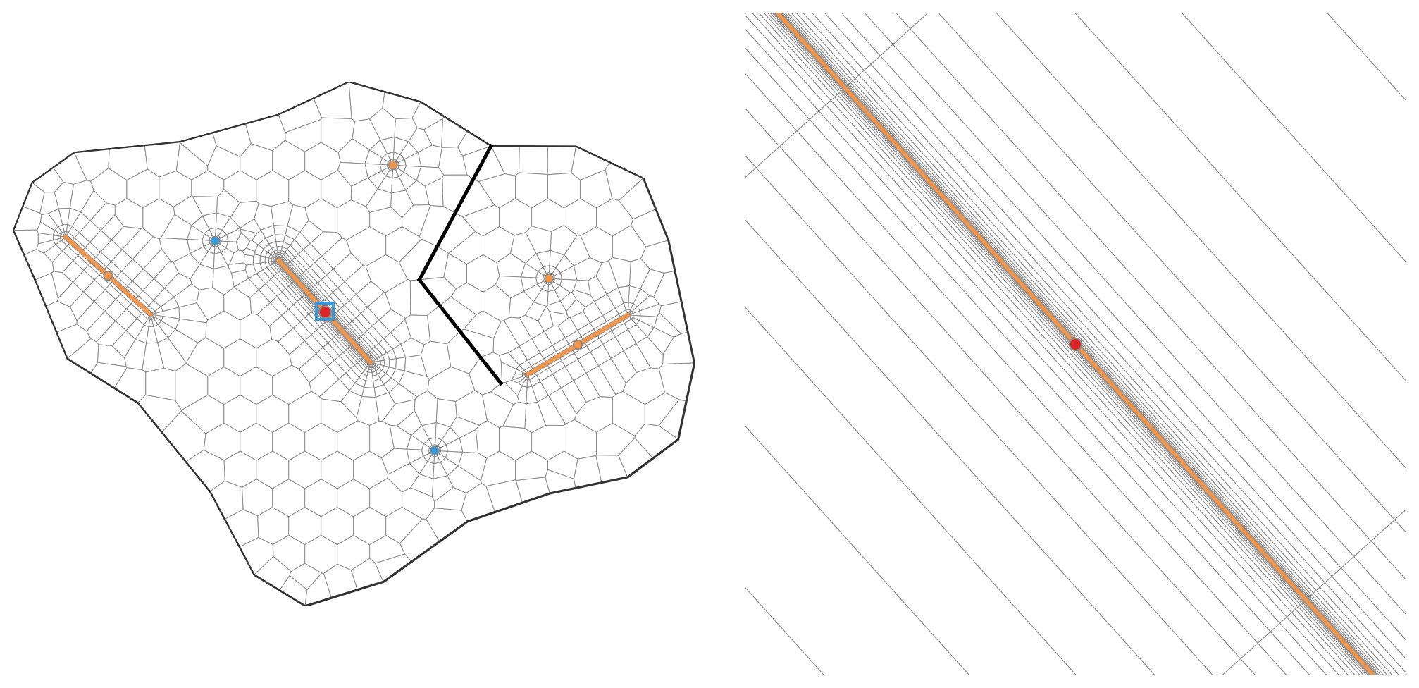
The main drawback is the effort required during preprocessing. The complexity shifts to the algorithms for placing the generating points. We need parametric well templates, rules for generating points along faults, and logic for resolving conflicts where complex objects intersect. The quality of the final grid depends entirely on how carefully these geometric rules are designed.
Testing simulation speed and accuracy
To assess which grid is better suited to well test interpretation in practice, we will run a comparison under the following conditions:
- We use the reservoir map from the grid overview and select one well as the study well.
- We check pressure accuracy only at the study well.
- We allow coarser cells in areas away from the main flow features until further coarsening starts to affect pressure at the study well.
- Our reference is a calculation of the same problem in a commercial simulator with its accuracy settings at their maximum.
- We compare the grids using two measures: deviation of the Bourdet derivative from the reference and calculation time.
We use the finite-volume method with fully implicit time discretization and a two-point flux approximation. For each grid type, we consider two contrasting grid generation settings:
- Accuracy first: a fine grid with a high level of detail, where calculation time is not a limiting factor.
- Speed first: a coarse grid with the minimum acceptable number of cells, where some loss of accuracy is accepted for faster calculation.
To assess how sensitive the methods are to the size and structure of the matrix, we also run each configuration with two types of linear solver: a direct solver using LU factorization and an iterative solver using BiCGSTAB with an ILU preconditioner.
Testing the detailed grids
We begin with the detailed grids shown in the overview. At this stage, we retain the detailed geometry and local refinement without trying to reduce the cell count for speed.
The conditions and time steps are identical for all grids. We compare calculation time and the root mean square relative error (RRMSE) of the Bourdet derivative. The derivative is more sensitive to changes in the response shape and transitions between flow regimes, so it better reflects distortions that matter for interpretation.
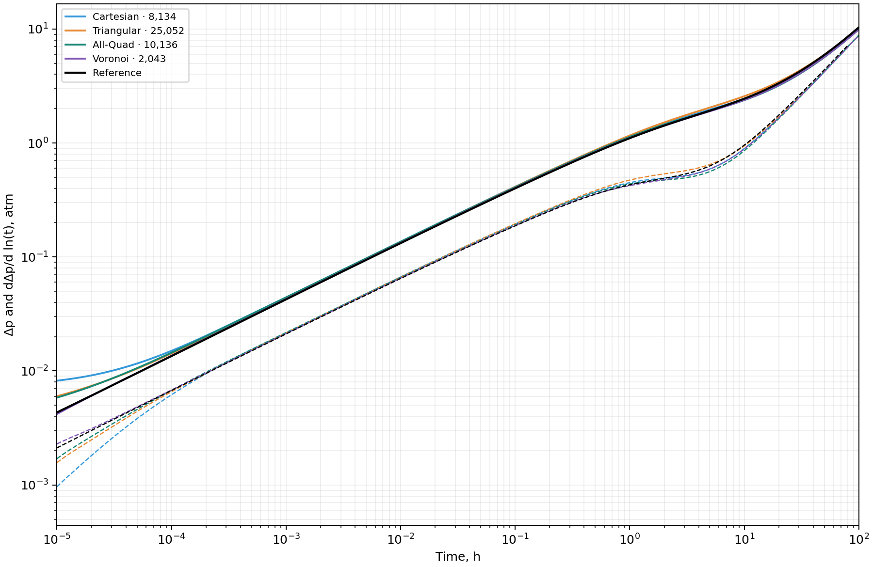
First, let's look at the curves. Overall, they reproduce the reference well, but artifacts are visible in two intervals. Early-time deviations are particularly pronounced and are associated with insufficient refinement around the study well. The second interval of divergence corresponds to the transition to boundary-dominated behavior. This also reflects the level of detail, this time in the reservoir boundary and surrounding objects.
The Voronoi grid stands out: its curves are visually closest to the reference.
Now let's look at the numerical results. The table reports the median time of three runs on one thread on the same computer. The timing includes solver setup, calculation, residual checks and material balance checks. It excludes grid generation, initial operator assembly and plotting.
| Grid | Cells | LU time, s | BiCGSTAB + ILU time, s | Derivative RRMSE, % |
|---|---|---|---|---|
| Cartesian | 8,134 | 4.294 | 1.613 | 13.25 |
| Triangular | 25,052 | 13.652 | 6.057 | 6.95 |
| All-Quad | 10,136 | 6.652 | 2.635 | 5.66 |
| Voronoi | 2,043 | 1.178 | 0.578 | 3.12 |
The Voronoi grid gives the lowest root mean square relative error of the derivative, at 3.12%, confirming its visual agreement with the reference. The triangular and All-Quad grids give errors of 6.95% and 5.66%. The Cartesian grid is noticeably less accurate, with an error of 13.25%. The numbers confirm what we have already seen on the plot.
The triangular grid has the most cells, at around 25,000. The All-Quad and Cartesian grids are considerably smaller and fairly close to each other, at around 10,000 and 8,000 cells. The Voronoi grid is the smallest, with only around 2,000 cells. Both solvers show the same trend: calculation speed clearly falls as the number of cells increases.
The Voronoi grid leads this test, calculating more accurately and faster with fewer cells. However, some of its speed advantage may come from excessive refinement in the other grids. Let's try to optimize them by reducing the number of cells in less active areas. We will keep the Voronoi grid as it is and see how the balance between speed and accuracy changes.
Testing the optimized grids
We optimize the Cartesian, triangular and All-Quad grids. Around the study well, we revise the refinement strategy, retaining local detail while removing unnecessary cells. We simplify the grids considerably around offset wells, reduce the detail along boundaries and faults, and use larger cells in less active areas. The Voronoi grid stays the same.
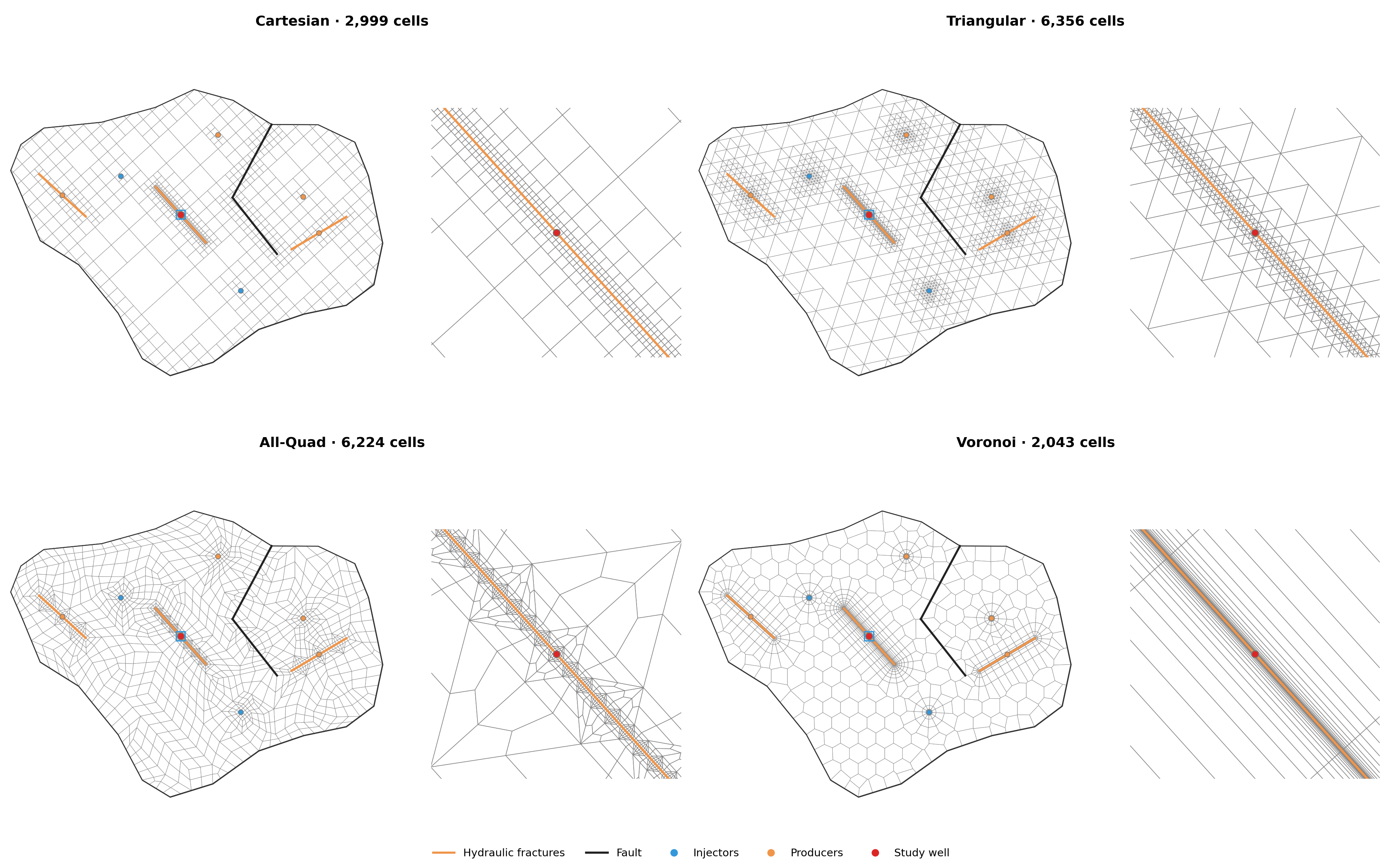
After optimization, the Cartesian cell count falls from 8,134 to 2,999, the triangular count from 25,052 to 6,356, and the All-Quad count from 10,136 to 6,224. The Voronoi grid retains its 2,043 cells. Further reductions noticeably degrade calculation accuracy, so we stop at these values.
We keep the calculation conditions, solvers and error measure the same. Let's see how coarsening has affected the pressure and derivative curves.
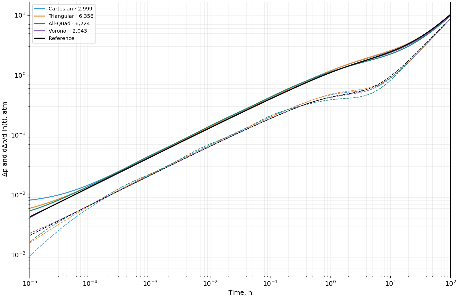
Early-time behavior has barely changed. Small wave-like artifacts have appeared during linear flow, most noticeably in the All-Quad grid's derivative. During the transition to boundary-dominated behavior, the artifacts become stronger because the surrounding area is represented more coarsely. The Voronoi curve stays the same because its grid has not changed.
Now for the metrics. As in the first test, the reported time is the median of three runs on one thread. The timing scope and comparison interval remain the same.
| Grid | Cells | LU time, s | BiCGSTAB + ILU time, s | Derivative RRMSE, % |
|---|---|---|---|---|
| Cartesian | 2,999 | 1.198 | 0.618 | 13.79 |
| Triangular | 6,356 | 2.462 | 1.264 | 7.57 |
| All-Quad | 6,224 | 3.255 | 1.585 | 9.53 |
| Voronoi | 2,043 | 1.178 | 0.578 | 3.12 |
Optimization has noticeably accelerated the calculation. The Cartesian grid is now very close to the Voronoi grid in speed, and the triangular and All-Quad grids also run substantially faster.
As expected, this speedup comes with a loss of accuracy, visible both in the curves and in the increase in derivative RRMSE. Further optimization becomes impractical: a small additional gain in speed comes at the cost of accuracy losses that are critical for well test interpretation.
Conclusion
The calculations show that, for well testing, the Voronoi grid clearly outperforms the alternatives in both speed and accuracy. Returning to the question at the start of the article, we can now see why this approach became the de facto standard in well testing.
Other grid types are considerably easier to implement. A Voronoi grid requires a comprehensive, carefully designed algorithm for placing the generating points, which raises the barrier to developing a numerical simulator. For a one-off research project, a simpler option such as an adaptive Cartesian grid can therefore be a reasonable choice. It provides acceptable accuracy without requiring extensive work on the grid generator's geometry.
For routine well test calculations, however, the best tool is needed. The volume of subsequent work pays back the investment in a complex grid generator. We use this approach to grid generation in our SiamWellTest software.