Goal. Walk through preparing input data for well test interpretation in SiamWellTest and show the tools that cover most situations when loading and reconciling pressures and rates.
Who it is for. This document is useful to three groups of readers:
- well test interpretation engineers who are starting to work in SiamWellTest or moving to it from other software: it shows how to do familiar data preparation in a new tool;
- well testing team leads who are evaluating software: it gives an idea of the effort needed for data preparation and how far the process can be standardized;
- reservoir engineers and geologists who use interpretation results: it shows how much work well test engineers do to obtain diagnostic plots.
What we do. Using a hypothetical oil well as an example, we go from scattered data sets to diagnostic plots:
- Loading the input data.
- Preparing the pressure.
- Preparing the rate history.
- Reconciling pressure and rates.
- Building and analyzing diagnostic plots.
Input data
For this case we take two typical well data sources: pressure from the ESP downhole gauge and rates from the monthly production report. Such data exist for almost any artificial-lift well, and they are what engineers work with most often. They are far from ideal, though: they come from different systems, differ in resolution, and do not always agree with each other. This lets us go through most of the situations that come up during data preparation and use most of the data preparation tools.
Pressure
The downhole gauge records pressure continuously, both while the well is producing and during shut-ins. The series is therefore dense and contains every well event, including those not reflected in other sources.
| Parameter | Value |
|---|---|
| Source | ESP downhole gauge |
| Recording period | 17.11.2022 – 01.06.2025 |
| Sampling | 1 min, 1 s during some shut-ins |
| Number of points | 160856 |
Rates
Rates come from periodic measurements taken from the production report. The rate is assumed constant between measurements. Shut-ins that happened between measurements may not appear in this data.
| Parameter | Value |
|---|---|
| Source | Production report |
| Period | 13.07.2023 – 02.06.2025 |
| Sampling | 1 day |
| Number of records | 690 |
Loading the input data
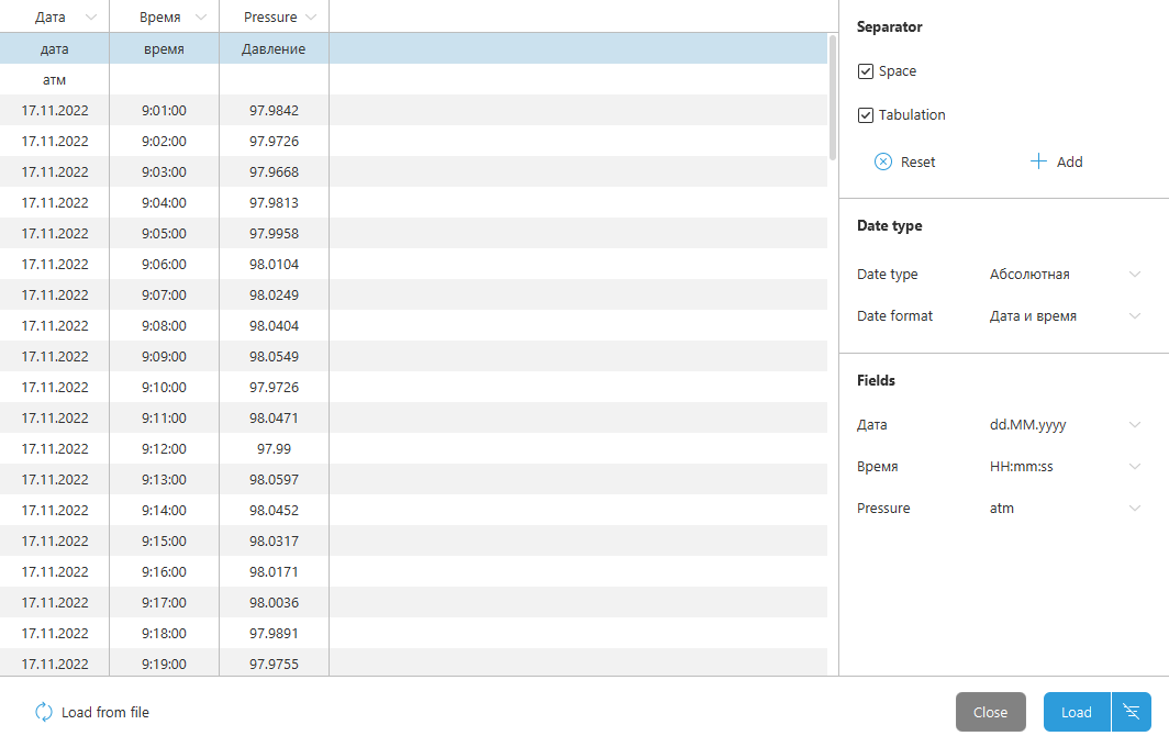
Pressure and rates are loaded through the text file loader. It parses delimited data, so there is no need to preprocess files in Excel or other programs. Both data sets are loaded the same way; below it is shown for pressure.
Steps:
- Select the file. Click "Load from file" and choose a text file. Its contents appear in the preview table right away, so you can see whether the data are parsed correctly.
- Separators. In the "Separator" block, check the characters that separate columns in the file: space, tab, or both. If the file uses another character, add it with the "Add" button. The preview table updates immediately and shows how the file is split into columns.
- Date type. Specify how time is recorded in the file. In our case it is absolute time: calendar date and time in
dd.MM.yyyyandHH:mm:ssformat. Time can also be set in relative format or as steps. - Units. In the "Fields" block, choose the units each parameter is recorded in, for example pressure in atm. There is no need to convert the data beforehand.
- Assign columns. In the header of each preview table column, choose what it contains: date, time, pressure. Leave columns you do not need unassigned.
Then click "Load".
The setup only needs to be done once. The loader remembers your last choices: separators, date type and format, units, and column assignment. Exports from the same system usually share one format within a company, so for the next files you only need to select the file and click "Load".
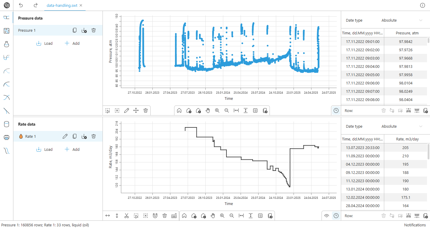
After loading, both series are shown on a common time axis, and you can immediately see how they relate to each other.
Initial review
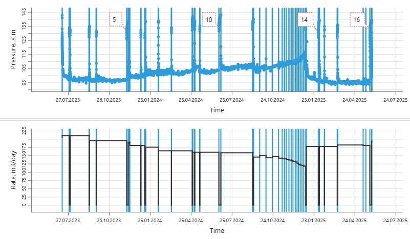
At first glance the pressure is clean: there are no obvious outliers, and the record is continuous over most of the period. The plot shows many well shut-ins, and each of them is a potential pressure build-up (PBU).
The rates, as expected from production report data, are of low quality. They do not cover the whole pressure recording period, and the shut-ins clearly visible on the pressure are not reflected in them.
As a result, the data have three problems:
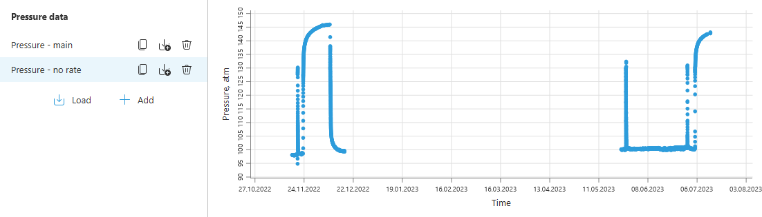
- There is a large gap in the pressure record: from 17.12.2022 to 24.05.2023.
- In the initial interval, from 17.11.2022 to 13.07.2023, there is pressure but no rates. It cannot be discarded: it contains two long PBUs.
- In the main interval, well shut-ins are not marked in the rate history.
Splitting the data into intervals
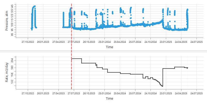
Rates do not cover the whole pressure recording period: the production report starts on 13.07.2023, while pressure is recorded from 17.11.2022. The simplest option would be to trim the pressure at the start of the rates and discard the rest. But the interval without rates contains two long PBUs that are useful for analysis. So we do not throw this interval away but treat it separately. The data are split into two intervals:
- main interval (13.07.2023 – 01.06.2025): both pressure and rates are available;
- no-rate interval (17.11.2022 – 13.07.2023): only pressure is available, but the data still carry information for analysis.
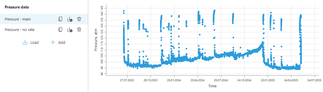
To keep the intervals from interfering with each other, make a copy of the pressure series. In the original, keep only the main interval: select the range before 13.07.2023 and delete those points. In the copy, do the opposite and keep only the no-rate interval. To avoid confusion later, rename the series, for example "Pressure - main" and "Pressure - no rate".
Marking shut-ins in the main interval
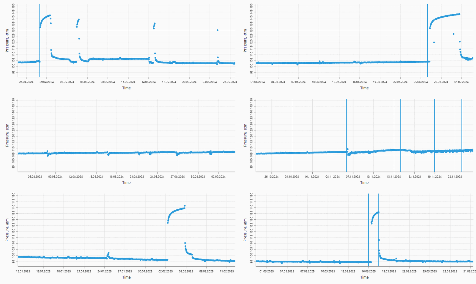
In the main interval the pressure is of good quality, but well shut-ins are not reflected in the rate history, even though they stand out clearly on the pressure plot.
Marking is done in three steps:
- Rough cutting. Use the "Scissors" tool to cut the rate history at the shut-ins. Precision does not matter here. Zoom and pan work with the mouse wheel, so you do not need to switch tools.
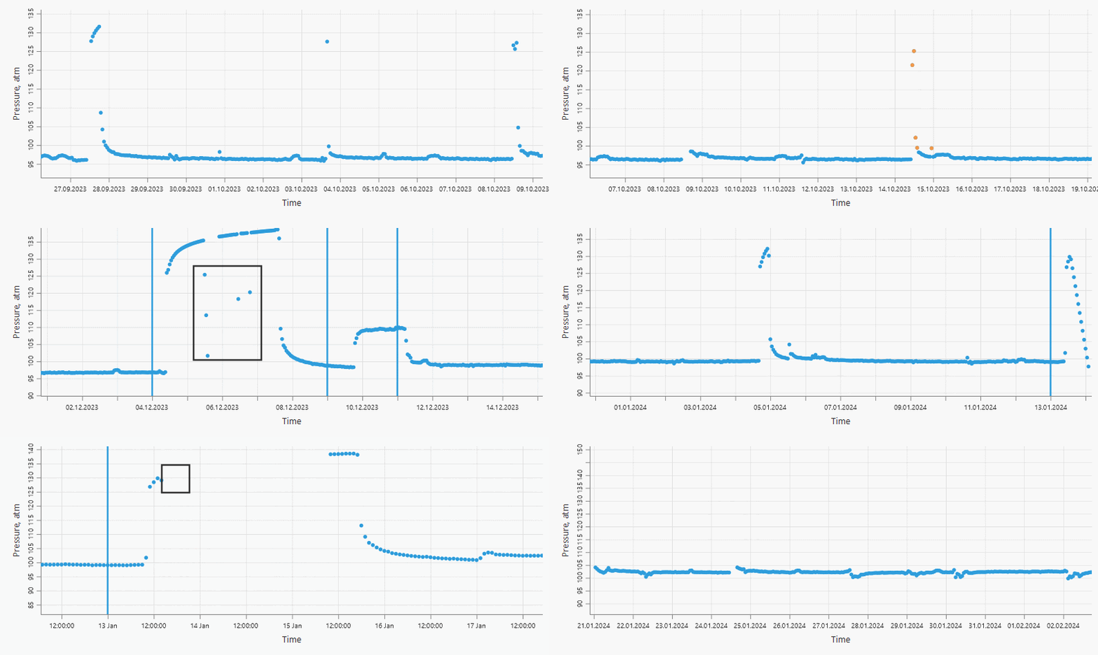
- Selecting shut-ins. Significant shut-ins, long and with enough points, were already marked in the previous step. Short shut-ins of 2–3 points are not marked; delete their pressure points instead: they carry no information for analysis and only clutter the plot.
- Fine adjustment. Using the horizontal editing tool with snapping to pressure points enabled, align the start of the period with the first point of the shut-in and the end with the last one. In the rate period table, set the rate on this interval to 0.
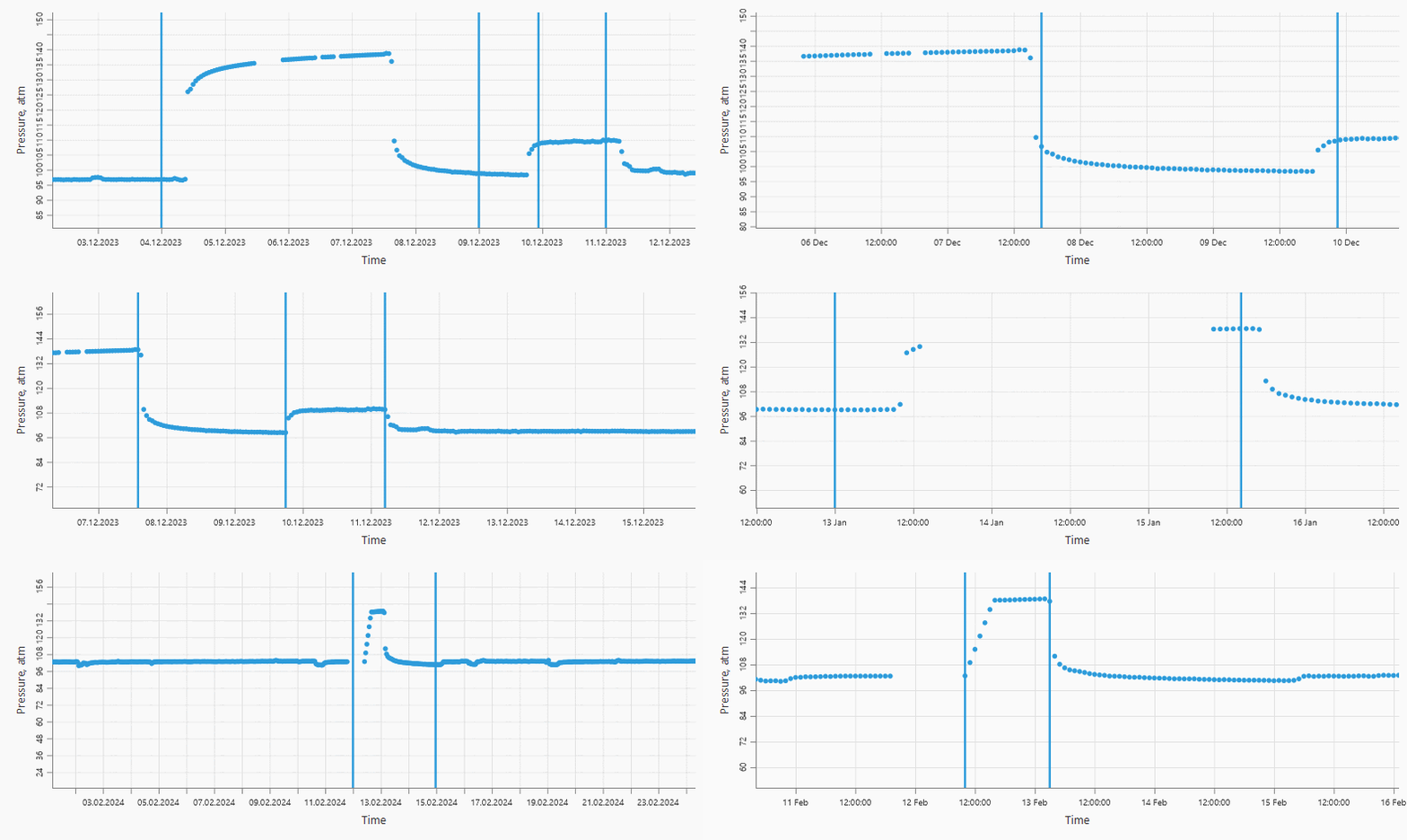
In total, 16 significant shut-ins were marked. Four of them, Nos. 5, 10, 14 and 16, are long enough to extract diagnostic plots from. The whole procedure took no more than 10 minutes.
Marking the no-rate interval
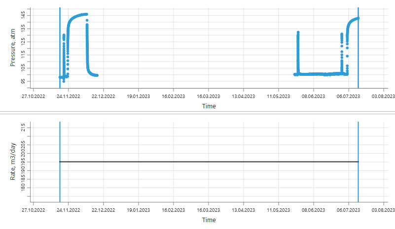
The interval 17.11.2022 – 13.07.2023 has pressure only. Suppose rates for this period cannot be obtained. The pressure shows that the reservoir behaves roughly the same as in the main interval: the flowing bottomhole pressure stays at 97–100 atm. So we assume the rate is close to the known values and create a new rate series with a constant value of 195 m³/d for the whole period.
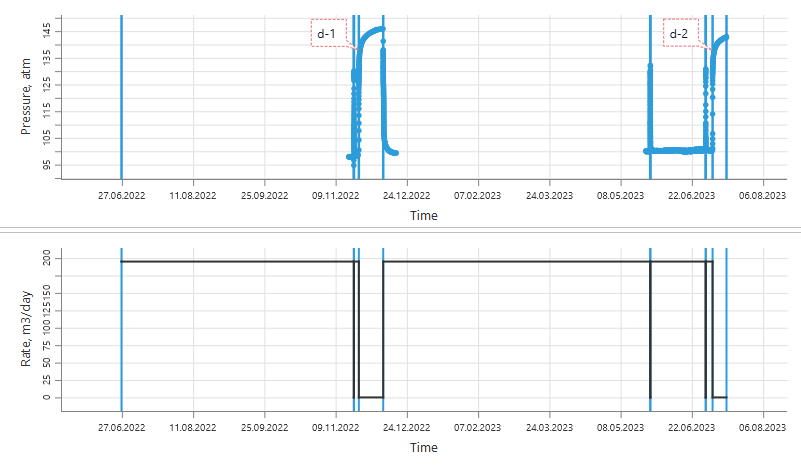
From here, marking goes the same way as in the main interval: rough cutting with scissors, then fine adjustment of the boundaries with snapping to pressure points.
The start of the history needs separate attention. The well was already producing when pressure recording began, so the start of the period is moved to the left, before the start of the data. If the rate history starts at the first pressure point, superposition will account for too short a production period before the PBU, and the derivative at late times will be distorted. The production period before the first PBU should be at least 5 times longer than the PBU itself.
Diagnostic plots
Diagnostics are extracted in the PTA module: select the pressure and rate series and specify the PBU interval. We start with shut-in No. 5 of the main interval.
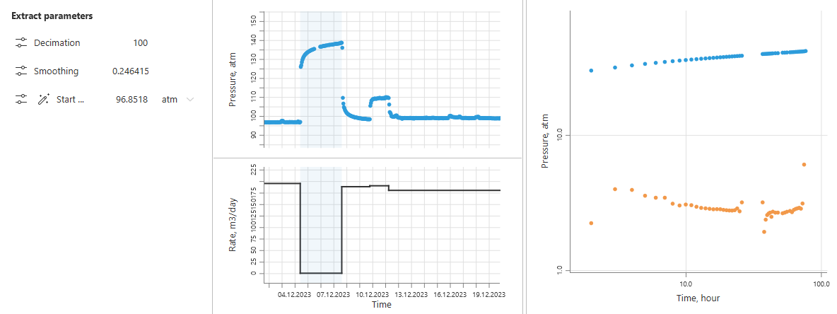
For the remaining PBUs, duplicate the analysis and change the extraction interval. This way we process shut-ins Nos. 10, 14 and 16 of the main interval and the two PBUs of the no-rate interval. Then in the comparison module we select all the analyses created and overlay their diagnostic plots.
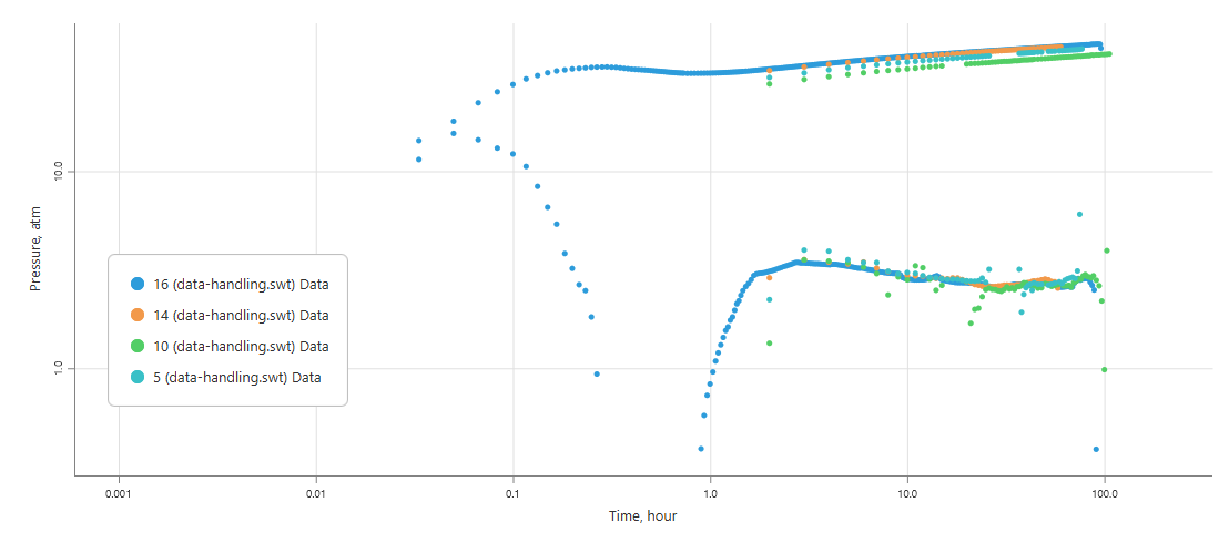
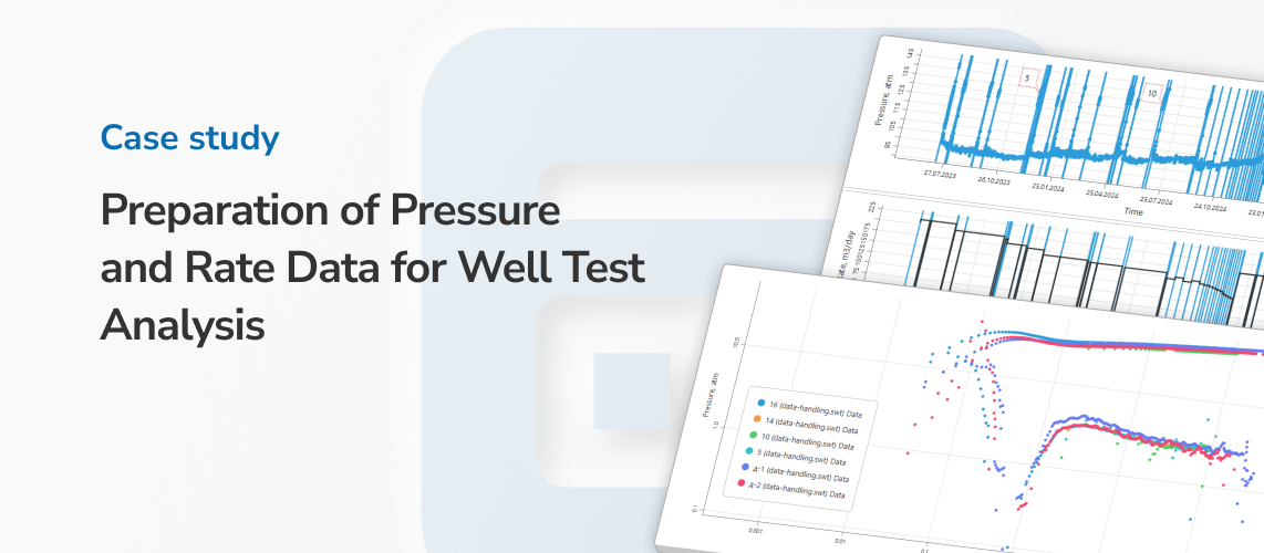
The plots match well in both pressure change and derivative: all PBUs show the same flow regimes at the same times. Three PBUs were recorded at 1-minute sampling, so they have no early-time data. On PBU No. 16 pressure was recorded every second, and it shows the early-time segment: the wellbore storage effect.
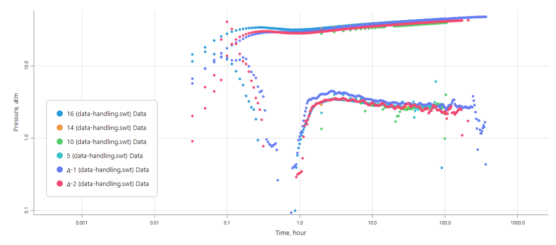
The PBUs of the no-rate interval fall in the same range as those of the main interval and repeat the same flow regimes. All six PBUs show the same reservoir response. They can therefore be interpreted together, and reservoir parameters can be checked against several independent shut-ins.
Conclusion
In this work we looked at typical field data, pressure from the ESP downhole gauge and rates from the production report, with their usual problems: noise in pressure, unmarked shut-ins and gaps in the rate history.
All the preparation was done in SiamWellTest, without processing files in third-party programs:
- Loading is set up once. After that, files of the same type load in a couple of clicks.
- Marking shut-ins in the main interval took no more than 10 minutes.
- Intervals without rates were treated separately: with a reasonable rate assumption, useful data were extracted from them too.
- Comparison of diagnostic plots showed excellent agreement of the prepared data.
This kind of data set is found on most artificial-lift wells, so the techniques shown apply to the everyday work of well testing engineers. The next step is interpreting the resulting PBUs, which we will cover in a separate case.